Degree Distribution

A property of the full-scale structure of a network that is typically investigated is the distribution of the network node degrees. We recall that the degree of a node is the number of neighbours of the node. For any integer $k \geq 0$, the quantity $p_k$ is the fraction of nodes having degree $k$. This is also the probability that a randomly chosen node in the network has degree $k$. The quantities $p_k$, for $k \geq 0$, represent the degree distribution of the network.

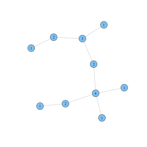
Consider for instance the following simple graph with 10 nodes. Nodes are labelled with their degree. The degree distribution is the following (notice that $p_k = 0$ for all $k \geq 5$):

$\displaystyle{p_0 = 0, p_1 = \frac{5}{10}, p_2 = \frac{3}{10}, p_3 = \frac{1}{10}, p_4 = \frac{1}{10} }$

Another construct containing the same information as the degree distribution is the degree sequence, which is the set $(k_1, k_2, \ldots, k_n)$ of degrees of the $n$ nodes labelled as $1, 2, \ldots, n$. For example, the degree sequence for the above graph is $(1, 1, 1, 1, 1, 2, 2, 2, 3, 4)$.

Directed networks have two different degree distributions, the in-degree and the out-degree distributions. Typically, the in-degree distribution is the important one. We might observe, however, that the true degree distribution of a directed network is a joint distribution of in- and out- degrees. That is, for every $i,j \geq 0$, we have a probability $p_{i,j}$ that a randomly chosen node in the graph has $i$ predecessor nodes and $j$ successor nodes. By using a joint distribution in this way we can investigate the correlation of the in- and out- degrees of vertices. For instance, if vertices with high out-degree tend to have also high in-degree.

It bears say that a knowledge of the degree distribution does not, in most cases, tell us the complete structure of a network. For most choices of degrees there is more than one network with those degrees.

In most real networks, the degree distribution is highly asymmetric (or skewed): most of the nodes (the trivial many) have low degrees while a small but significant fraction of nodes (the vital few) have an extraordinarily high degree. A highly connected node, a node with remarkably high degree, is called hub. Since the probability of hubs, although low, is significant, the degree distribution $p_k$, when plotted as a function of the degree $k$, shows a long tail, which is much fatter than the tail of a Gaussian or exponential model.

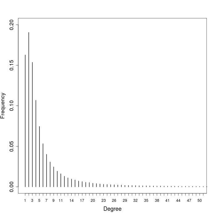
Consider, for instance, the degree distribution for the collaboration network in computer science, depicted in the next histogram. The distribution has in fact a long tail: roughly half of the scholars have one, two, or three unique collaborators. The other half of the scholars distribute over a slow decreasing long tail. There are, for instance, 350 scholars with 50 collaborators, and 40 scholars with 100 collaborators. The tail is in fact longer than shown in the figure, with 28 authors with more than 300 collaborators and the most collaborative computer scientist with 595 unique co-authors.

This asymmetric shape of the degree distribution has important consequences for the processes taking place on networks. The highly connected nodes, the hubs of the network, are generally responsible for keeping the network connected. In other words, the network falls apart if the hubs are removed from the network. On the other hand, since hubs are rare, a randomly chosen node is most likely not a hub, and hence the removal of random nodes from the network has a negligible effect on the network cohesion. Substantially, networks with long tail degree distributions are resilient to random removal of nodes (failure) but vulnerable to removal of the the hub nodes (attack).

Hubs are also important for the spread of information or of any other quantity flowing on the network. In fact, hubs play a dual role in information diffusion over the network: on the one hand, since they are highly connected, they quickly harvest information, on the other hand, and for the same reason, they effectively spread it. In a network with hub nodes, the probability that each node spreads the information to its neighbours need not be large for the information to reach the whole community.

To quantitatively study the asymmetry of the degree distribution, one can investigate the skewness and the concentration of the distribution. Skewness measures the symmetry of a distribution. A distribution is symmetric if the values are equally distributed around its mean, it is right skewed if it contains many low values and a relatively few high values, and it is left skewed if it comprises many high values and a relatively few low values. As a rule of thumb, when the mean is larger than the median the distribution is right skewed and when the median dominates the mean the distribution is left skewed. For instance, the mean degree for the computer science collaboration network is 6.63, and the median degree is 3.

A numerical indicator of skewness of the distribution of a random variable $X$ with mean $\mu$ and standard deviation $\sigma$ is the third standardized central moment of the distribution: $$\gamma_1 = E \left[\left(\frac{X - \mu}{\sigma}\right)^3 \right]$$ Positive values for the skewness indicator correspond to right skewness (since there are outliers far above the mean), negative values correspond to left skewness (since there are outliers far below the mean), and values close to 0 mean symmetry. The skewness indicator for the computer science collaboration graph is 8.04.

Concentration measures how the character is equally distributed among the statistical units. The two extreme situations are equidistribution, in which each statistical unit receives the same amount of character and maximum concentration, in which the total amount of the character is attributed to a single statistical unit. A typical example of use of concentration is the allocation of wealth among individuals since it seemed to show rather well the way that a larger portion of the wealth of any society is owned by a smaller percentage of the people in that society.

A useful representation of concentration is the Lorenz concentration curve. This is obtained by sorting the statistical units (e.g., people) in decreasing order with respect to the amount of character they own (e.g., income). Then, the share of top units collecting a given percentage of character is plotted. The Lorenz curve can be used to investigate the concentration of the edges among nodes in a network, that is the asymmetry of the degree distribution. If edges are equally distributed among nodes, then all nodes have roughly the same degree, and the degree distribution is symmetric. If, however, a significant share of edges is concentrated on few highly connected nodes, then the degree distribution is right skewed. By way of example, here is the Lorenz curve for the collaboration in computer science.

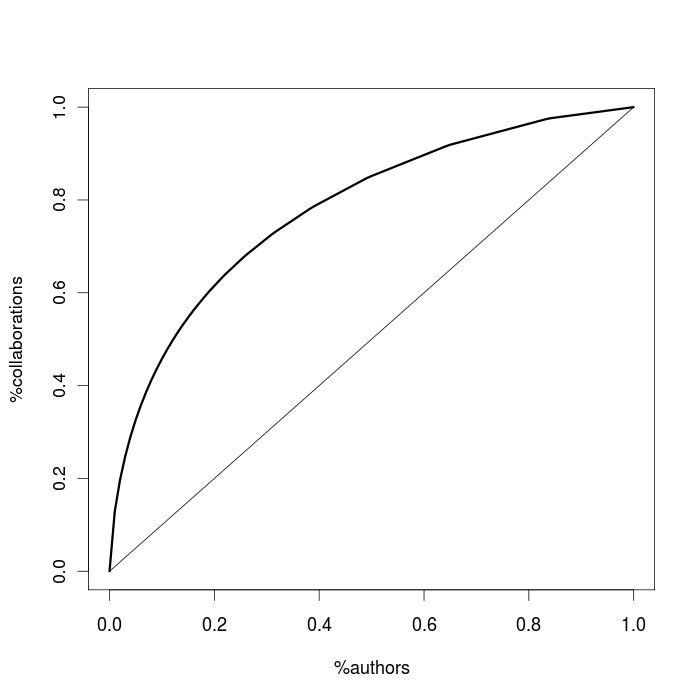
It is clear that the concentration of collaboration is far from the equidistribution situation, which is illustrated by the straight line with slope 1. For instance, the most collaborative 1% of the scholars harvest 13% of the collaborations, the 5% of them collect one-third (33%) of the collaborations, and the 10% of them attract almost half (46%) of the collaborations.

A numerical indicator of concentration is the Gini coefficient, which is the ratio of the area contained between the concentration curve and the equidistribution line and the area representing maximum concentration. The index ranges between 0 and 1 with 0 representing equidistribution and 1 representing maximum concentration. For instance, the Gini coefficient is 0.56 for the computer science collaboration network.

To be sure, the most popular long tail probability distribution is the power law. For a degree distribution, it states that the probability $p_k$ of having a node with $k$ neighbours is $$p_k = C k^{-\alpha}$$ where $C$ is a normalization constant and $\alpha$ is known as the exponent of the power law. Values in the range $2 \leq \alpha \leq 3$ are typical for degree distributions networks. Notice that, taking the logarithm of both members of the power law definition, we have:

An alternative (and more convenient) method to visualize and detect a power law behaviour is to plot the complementary cumulative distribution function (CCDF) on log-log scales. The CCDF $P_k$ is the fraction of vertices that have degree $k$ or greater: $$P_k = \sum_{x = k}^{\infty} p_{x}$$

Notice that, if $p_k = C k^{-\alpha}$ and $\alpha > 1$, then:

It follows that if a distribution follows a power law, then so does the CCDF of the distribution, but with exponent one less than the original exponent. Hence, when plotted on log-log scales, the CCDF of a power law should appear as a straight line. For example, the next plot shows the CCDF for the computer science collaboration network. Notice that the curve shows a clear upward curvature, a sign that it does not match the power law model on the entire domain.

In practice, few empirical phenomena obey power laws on the entire domain. More often the power law applies only for values greater than or equal to some minimum location. In such case, we say that the tail of the distribution follows a power law. Networks that have a power law degree distribution are sometimes called scale-free networks. The name comes from the fact that, as opposed to random networks, scale-free networks possess no characteristic scale, meaning that there is no typical node in the network that represents the degree for the other nodes.

Clauset et al. developed a principled statistical framework for discerning and quantifying power law behaviour (the interested reader can read Fitting empirical distributions to theoretical models). We applied the techniques developed by them to detect a power law behaviour in the degree distribution of the computer science collaboration network. As expected, the degree distributions do not follow a power law on the entire regime. Nevertheless, the degree distribution for the whole collaboration network has a power law tail starting from degree 111 ($\alpha = 4.4$, p-value = 0.11). The tail contains, however, only 1098 highly collaborative scholars, which correspond to 0.16% of all authors.

As for the network models, consider a random graph with $n$ nodes and edge probability $p$. The probability $p_k$ that a node has $k$ neighbours is the binomial $$p_k = {n \choose k} p^k (1-p)^{n-1-k}$$ which can be approximated by the Poisson distribution $$p_k = \frac{\lambda^k e^{-\lambda}}{k!}$$ for large values of $n$ and small values of $p$, where $\lambda = p(n-1)$ is the mean degree of a node in the network. The Poisson distribution is peaked at the average degree $\lambda$: the majority of nodes have the same typical degree and nodes deviating from the average are extremely rare. In other words, a random network has a characteristic scale, which contrasts with the scale-free nature of real webs. On the other hand, the degree distribution of a graph generated with the preferential attachment model asymptotically follows a power law distribution with exponent parameter $\alpha = 3$. Hence, this model is more realistic than the random one.