The goal is fitting an observed empirical data sample to a theoretical distribution model. The fitting problem can be split in three main tasks:
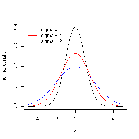
Popular examples of theoretical distributions are normal (Gaussian), lognormal, and power law (Pareto). The normal distribution has density:
$\displaystyle{f(x) = \frac{1}{\sqrt{2 \pi} \sigma} e^{-\frac{(x - \mu)^2}{2 \sigma^2}}}$
where $\mu$ is the mean of the distribution and $\sigma$ the standard deviation.
plot(function(x) {dnorm(x)}, -5, 5, ylab="normal density")
plot(function(x) {dnorm(x, sd=1.5)}, -5, 5, col="red", add=TRUE)
plot(function(x) {dnorm(x, sd=2)}, -5, 5, col="blue", add=TRUE)
legend(x = "topleft", legend = c("sigma = 1", "sigma = 1.5", "sigma = 2"),  lty = c(1, 1, 1), col = c("black", "red", "blue"))
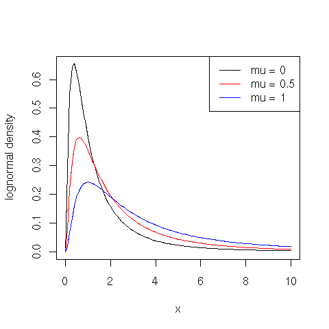
The lognormal probability density function is defined for $x > 0$ in terms of parameters $\mu$ and $\sigma > 0$ as follows:
$\displaystyle{f(x) = \frac{1}{\sqrt{2 \pi} \sigma x} e^{-\frac{(\log(x)-\mu)^2}{2 \sigma^2}}}$
plot(function(x) {dlnorm(x, meanlog = 0)}, 0, 10, ylab="lognormal density")
plot(function(x) {dlnorm(x, meanlog = 0.5)}, 0, 10, col="red", add=TRUE)
plot(function(x) {dlnorm(x, meanlog=1)}, 0, 10, col="blue", add=TRUE)
legend(x = "topright", legend = c("mu = 0", "mu = 0.5", "mu = 1"),  lty = c(1, 1, 1), col = c("black", "red", "blue"))
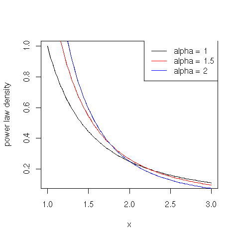
The probability density function for a power law distribution is defined for $x \geq x_0 > 0$ in terms of the scaling exponent parameter $\alpha > 0$ as follows:
$\displaystyle{f(x) = \frac{\alpha \, x_{0}^{\alpha}}{x^{\alpha + 1}}}$
Normal and lognormal distribution functions are already encoded in R (use suffixes norm and lnorm, respectively). In the following we code in R the power law distribution functions with exponent shape and minimum value location:
dpareto=function(x, shape=1, location=1) shape * location^shape / x^(shape + 1);
ppareto=function(x, shape=1, location=1) (x >= location) * (1 - (location / x)^shape);
qpareto=function(u, shape=1, location=1) location/(1 - u)^(1 / shape);
rpareto=function(n, shape=1, location=1) qpareto(runif(n), shape, location);
plot(function(x) {dpareto(x, shape = 1)}, 1, 3, ylab="power law density")
plot(function(x) {dpareto(x, shape = 1.5)}, 1, 3, col="red", add=TRUE)
plot(function(x) {dpareto(x, shape = 2)}, 1, 3, col="blue", add=TRUE)
legend(x = "topright", legend = c("alpha = 1", "alpha = 1.5", "alpha = 2"),  lty = c(1, 1, 1), col = c("black", "red", "blue"))
The maximum likelihood estimation method (MLE) is the most popular method to estimate the distribution parameters from an empirical sample. It finds the model parameters that maximize the likelihood of the observed data with respect to the theoretical model. For most distributions, the MLE parameters have a closed form:
# MLE for normal distribution d
mean = mean(d)
sd = sd(d)

# MLE for lognormal distribution d
meanlog = mean(log(d))
sdlog = sd(log(d))

# MLE for power law distribution d (continuous case)
shape = 1 / mean(log(d / location))

# MLE for power law distribution d (discrete case)
shape = 1 / mean(log(d / (location - 0.5)))
The shape parameter for the power law distribution in the discrete case in an approximate expression using the approach in which true power-law distributed integers are approximated as continuous power-law distributed reals rounded to the nearest integer. The estimation for the location parameter of the power law is more involved and will be considered later. If no closed form exists for the parameters, one has to find the parameters by maximizing the likelihood function with numerical methods. The MASS package contains a fitdistr function that does the job:
mle = fitdistr(d, "lognormal")
meanlog = mle$estimate["meanlog"]
sdlog = mle$estimate["sdlog"]
Let's come to the tricky step that establishes how good the observed data match the theoretical model with the estimated parameters. You may use the Shapiro-Wilk test to fit normal distributions. If the p-value is lower than a threshold (usually fixed to 0.05), than the normality hypothesis is rejected:
> shapiro.test(rnorm(100, mean = 5, sd = 3))

        Shapiro-Wilk normality test

data:  rnorm(100, mean = 5, sd = 3)
W = 0.9916, p-value = 0.795

> shapiro.test(runif(100, min = 2, max = 4))

        Shapiro-Wilk normality test

data:  runif(100, min = 2, max = 4)
W = 0.9605, p-value = 0.004379
To fit an arbitrary distribution, use the Kolmogorov-Smirnov test. The KS test compares an empirical and a theoretical model by computing the maximum absolute difference between the empirical and theoretical distribution functions:
$\displaystyle{D = \max_x |\hat{F}(x) - F(x)|$where $\hat{F}(x)$ is the empirical distribution function (the relative frequency of observations that are smaller than or equal to $x$), and $F(x) = P(X \leq x)$ is the theoretical distribution function.
> ks.test(rlnorm(100, meanlog = 2, sdlog = 1), plnorm, meanlog = 2, sdlog = 1)

        One-sample Kolmogorov-Smirnov test

data:  rlnorm(100, meanlog = 2, sdlog = 1)
D = 0.1075, p-value = 0.198
alternative hypothesis: two-sided

> ks.test(rlnorm(100), pnorm)

        One-sample Kolmogorov-Smirnov test

data:  rlnorm(100)
D = 0.5559, p-value < 2.2e-16
alternative hypothesis: two-sided
Again, if the p-value is lower than a given threshold, than the goodness-of-fit hypothesis is rejected. You may use the KS test also to check whether two datasets come from the same distribution:
> ks.test(rnorm(100), rnorm(100))

        Two-sample Kolmogorov-Smirnov test

data:  rnorm(100) and rnorm(100)
D = 0.08, p-value = 0.9062
alternative hypothesis: two-sided

> ks.test(rnorm(100), rnorm(100, mean = 1))

        Two-sample Kolmogorov-Smirnov test

data:  rnorm(100) and rnorm(100, mean = 1)
D = 0.57, p-value = 1.554e-14
alternative hypothesis: two-sided
Unfortunately, the fitness significance (p-value) computed by the Kolmogorov-Smirnov test is known to be biased if the parameters of the theoretical model are not fixed but, instead, they are estimated from the observed data. In particular, the computed p-value is overestimated, hence we run the risk of accepting the fitting hypothesis also when the data does not really come from the theoretical distribution.
To overcome this problem, A. Clauset and C. R. Shalizi and M. E. J. Newman recently proposed a methodology in their paper entitled Power-law distributions in empirical data, appeared in 2009 in SIAM Review. The proposed method reads as follows:
Clauset et al. suggest to reject the hypothesis of goodness of fit of the observed data with respect to the theoretical model if the p-value is lower than 0.1, that is, if less than 10% of the time the distance of the observed data from the model is dominated by the very same distance for synthetic data. The authors also claim that 2500 synthetic data sets are sufficient to guarantee that the p-valued is accurate to 2 decimal digits. Let's work the method out in R:
# Fits an observed distribution with respect to a lognormal model and computes p value
# using method described in:
# A. Clauset, C. R. Shalizi, M. E. J. Newman. Power-law distributions in empirical data.
# SIAM Review 51, 661-703 (2009)
# INPUT:
#   d: the observed distribution to fit
#   limit: the number of synthetic data sets to generate
# OUTPUT
#   meanlog: the meanlog (mu) parameter
#   sdlog: the sdlog (sigma) parameter
#   stat: the KS statistic
#   p: the percentage of time the observed distribution has a KS statistic lower than
#      or equal to the synthetic distribution
#   KSp: the KS p-value
lognormal = function(d, limit=2500) {

  # load MASS package to use fitdistr
  # mle = fitdistr(d, "lognormal");
  # meanlog = mle$estimate["meanlog"];
  # sdlog = mle$estimate["sdlog"];

  # MLE for lognormal distribution
  meanlog = mean(log(d));
  sdlog = sd(log(d));

  # compute KS statistic
  t = ks.test(d, "plnorm", meanlog = meanlog, sdlog = sdlog);

  # compute p-value
  count = 0;
  for (i in 1:limit) {
    syn = rlnorm(length(d), meanlog = meanlog, sdlog = sdlog);
    meanlog2 = mean(log(syn));
    sdlog2 = sd(log(syn));
    t2 = ks.test(syn, "plnorm", meanlog = meanlog2, sdlog = sdlog2);
    if(t2$stat >= t$stat) {count = count + 1};
  }

  return(list(meanlog=meanlog, sdlog=sdlog, stat = t$stat, p = count/limit, KSp = t$p));

}
Let fit a lognormal sample to a lognormal model:
> lognormal(rlnorm(1000), limit=100)
$meanlog
[1] 0.06426308

$sdlog
[1] 0.9751758

$stat
        D
0.0237101

$p
[1] 0.23

$KSp
[1] 0.6275387
As predicted, the p-value computed by Clauset et al. method is smaller than Kolmogorov-Smirnov p-value. Let's test whether citations received by Computer Science journal papers come from a lognormal model:
cites = scan("cscites.txt", 0)
cites = cites[cites > 0];

> lognormal(cites, limit=100)
$meanlog
[1] 1.828242

$sdlog
[1] 1.250804

$stat
         D
0.08194687

$p
[1] 0

$KSp
[1] 0
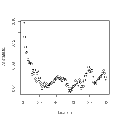
In the following we want to apply the Clauset et al. method to fit an observed sample to a power law model. However, we still have a question to answer: how do we estimate the location parameter of the model? In practice, few empirical phenomena obey power laws on the entire domain. More often the power law applies only for values greater than or equal to some minimum $x_0$. In such case, we say that the tail of the distribution follows a power law. For the estimation of the location parameter of a power law model, that is the starting value $x_0$ of the distribution tail, Clauset et al. propose to choose the value of $x_0$ that makes the empirical probability distribution and the best-fit power law model as similar as possible beginning from $x_0$. They use the KS statistic to gauge the distance between the observed data and the theoretical ones. We coded in R this method as follows:
# Fits an observed distribution with respect to a Pareto model using method described in:
# A. Clauset, C. R. Shalizi, M. E. J. Newman. Power-law distributions in empirical data.
# SIAM Review 51, 661-703 (2009)
# INPUT:
#   d: the distribution to fit
#   max: the maximum tested location value
# OUTPUT
#   fitting parameters and KS statistic and p-value (not reliable) for the fitting
#   with the lowest KS statistic plus vectors of all KS statistics and p-values

location = function(d, max=100)  {
 stat = NULL;
 p = NULL;
 mstat = 1;
 mp = NULL;
 mlocation = NULL;
 mshape = NULL;
 for (location in 1:max) {
   d = d[d >= location];
   # MLE for shape parameter (discrete case)
   shape = 1 / mean(log(d / (location - 0.5)));
   t = ks.test(d, "ppareto", shape = shape, location = location);
   stat[location] = t$stat;
   p[location] = t$p;
   if (stat[location] < mstat) {
     mstat = stat[location];
     mp = p[location];
     mlocation = location;
     mshape = shape;
   }
 }
 return(list(stat=mstat, p=mp, shape=mshape, location=mlocation, statvec=stat, pvec=p));
}
Here are the best fit parameters for the Computer Science citation data set:
par = location(cites)

> par$shape
[1] 1.800148

> par$location
[1] 56

> par$stat
[1] 0.03357657

> par$p
[1] 0.8183608

> min(par$statvec)
[1] 0.03357657

> which.min(par$statvec)
[1] 56

plot(par$statvec, xlab="location", ylab="KS statistic")
We are finally ready to code the Clauset et al. method to fit the tail of an observed sample to a power law model:
# Fits an observed distribution with respect to a Pareto model and computes p value
# using method described in:
# A. Clauset, C. R. Shalizi, M. E. J. Newman. Power-law distributions in empirical data.
# SIAM Review 51, 661-703 (2009)
# INPUT:
#   d: the observed distribution to fit
#   max: the maximum tested location value
#   limit: the number of synthetic data sets to generate
# OUTPUT
#   shape: the exponent parameter
#   location: the scale (minimum value) parameter
#   stat: the KS statistic
#   p: the percentage of time the observed distribution has a KS statistic lower than
#      or equal to the synthetic distribution
#   KSp: the KS p-value
pareto = function(d, max=100, limit=2500) {

  par = location(d, max);
  shape = par$shape;
  location = par$location;
  t = ks.test(d[d>=location], "ppareto", shape = shape, location = location);

  ntail = length(d[d>=location]);
  head = d[d < location];
  count = 0;
  for (i in 1:limit) {
    syn = rpareto(ntail, shape = shape, location = location);
    syn = c(head, syn);
    par2 = location(syn, max);
    shape2 = par2$shape;
    location2 = par2$location;
    t2 = ks.test(syn[syn >= location2], "ppareto", shape = shape2, location = location2);
    if(t2$stat >= t$stat) {count = count + 1};
  }

  return(list(shape=shape, location=location, stat = t$stat, p = count/limit, KSp = t$p));
}
Let's check whether there is a tail of the citation distribution for Computer Science papers that follows a power law:
> pareto(cites, 100, 100)
$shape
[1] 1.800148

$location
[1] 56

$stat
         D
0.03357657

$p
[1] 0.48

$KSp
[1] 0.8183608
Interestingly, the sample of citations greater than or equal to 56 nicely follows a power law model with exponent parameter $\alpha = 1.8$. Let's check the absolute and relative sizes of the power law tail:
> length(cites[cites >= 56])
[1] 355

> length(cites[cites >= 56]) / length(cites)
[1] 0.04927818