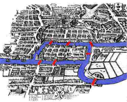
Köningsberg was a thriving city close to St. Petersburg in eastern Prussia on the banks of the Pregel. The city had seven bridges across the river, and its peaceful citizens wondered if one could ever walk across all seven bridges and never cross the same one twice. In 1736, Leonhard Euler modelled the Köningsberg bridge problem as a graph and mathematically showed that it has no solution. He argued that nodes with an odd degree must be either the start or the end point of an Eulerian path that traverses all bridges once. Hence, an Eulerian path cannot exist if the graph has more than two nodes with odd degree, which was the case for the Köningsberg bridge network.
Euler is credited as the father of graph theory and the Köningsberg bridge network as the first example of a graph. Besides solving the riddle, Euler unintentionally showed that networks have properties, which dependent on their topological architecture, that limit or enhance their usability.
Network analysis studies properties at three levels of abstraction:
In the following we will focus on undirected unweighted graphs. All network properties, however, can be generalized to directed as well as weighted graphs.
Centrality measures are indicators of the importance (status, prestige, standing, and the like) of a node in a network.
The simplest of centrality measure is degree centrality. Let $L$ be the adjacency matrix of a graph, that is, $l_{i,j} = 1$ if there is an edge from $i$ to $j$ in the graph and $l_{i,j} = 0$ otherwise. The degree $d_j$ of a node $j$ is the number of edges attached to it, that is:
$\displaystyle{d_j = \sum_i l_{i,j}}$
Nodes with high degree are called hubs and usually play an important role in the complex system modelled by the network.
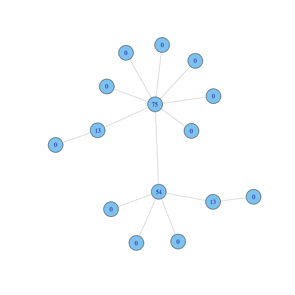
Consider the following scale-free graph:
g = barabasi.game(15, directed=FALSE)
coords = layout.fruchterman.reingold(g)

plot(g, layout=coords)
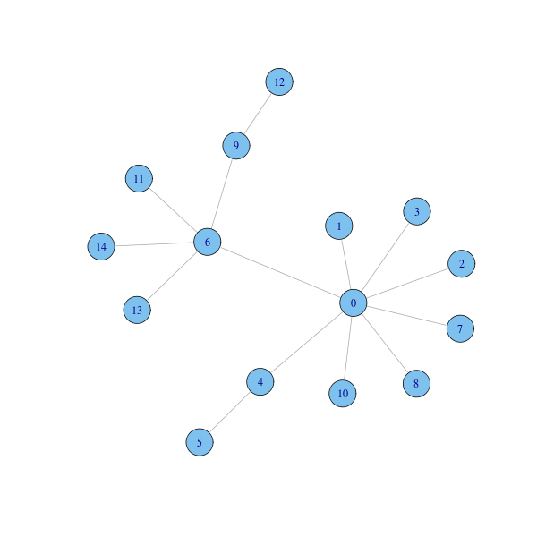
The degree function can be used to compute the degree of graph nodes:
degcent = degree(g)

names(degcent) = 0:(vcount(g) - 1)

sort(degcent, dec=TRUE)

 0  6  4  9  1  2  3  5  7  8 10 11 12 13 14
 8  5  2  2  1  1  1  1  1  1  1  1  1  1  1
A deeper measure is eigenvector centrality. The eigenvector centrality $p_j$ of node $j$ is recursively defined as:
$\displaystyle{p_j = \frac{1}{\lambda} \sum_i l_{i,j} p_i}$
where $\lambda \neq 0$ is a constant. In words, the eigenvector centrality of node $j$ is proportional to the sum of the centralities of neighbours of $i$. Hence, a node is important if it connected to other important nodes. In matrix notation, the eigenvector centrality equation reads $\lambda p = p L$, hence the centrality vector $p$ is the left-hand eigenvector of matrix $L$ associated to the eigenvalue $\lambda$.
However, a square matrix of size $n$ might have up to $n$ different real eigenvalues. Which value should one use? The dominant one, that is, the largest is absolute value. This choice guarantees nice properties. If $L$ is irreducible, that is if the network associated with $L$ is connected, and $\lambda$ is the dominant eigenvalue, then, by virtue of Perron-Frobenius Theorem, the eigenvector centrality equation has a positive and unique solution. In particular, positiveness avoids ties of the centrality scores at 0, which limit the discriminating power of the measure.
The well-known iterative power method can be used to computed an approximated value for the centrality vector. The convergence speed of the method is the rate at which $(\lambda_2 / \lambda_1)^k$ goes to $0$, where $\lambda_1$ and $\lambda_2$ are, respectively, the dominant and the sub-dominant eigenvalues of $L$, and $k$ is the number of iterations of the power method.
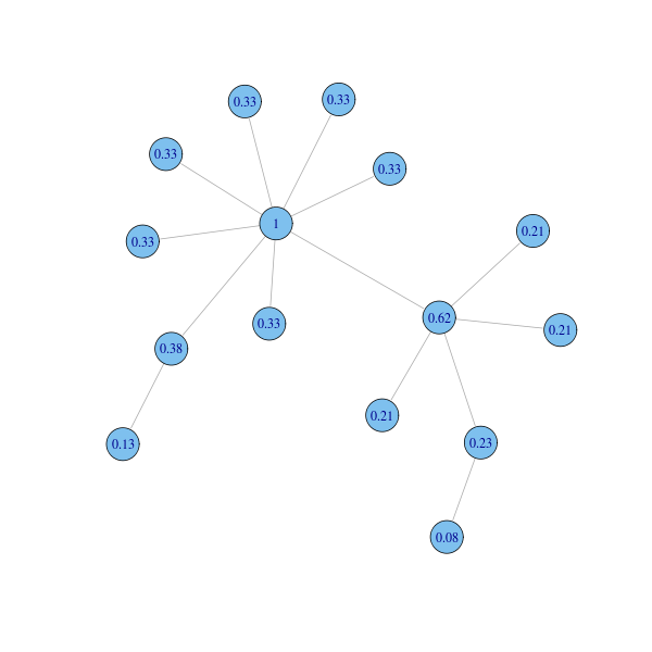
Function evcent computes the node eigenvector centrality:
eigcent = evcent(g)$vector

plot(g, layout=coords, vertex.label=round(eigcent, 2))
Alternative centrality measures are based on the notion of geodesic. Geodesy is a branch of geology measuring the size and shape of Earth. In the presence of a metric, a geodesic is a shortest path between points of the space, and the geodesic distance is the length of the geodesic. On a graph, a geodesic between two nodes is a path connecting the nodes with the smallest number of edges.
The closeness centrality $c_i$ of a node $i$ in a graph is the inverse of the mean geodesic distance from $i$ to every other node in the network:
$\displaystyle{c_i = \frac{n-1}{\sum_{j \neq i} d(i,j)}}$
where $d(i,j)$ is the geodesic distance between nodes $i$ and $j$ and $n$ is the number of nodes of the graph. If there is no path between nodes $i$ and $j$ then the total number $n$ of vertices is used in the formula instead of the path length.
Closeness lies in the interval $[0,1]$: nodes with closeness approaching 1 are nodes with short distance from the other nodes, while nodes with low closeness are distant from the other nodes. For instance, if a node is directly connected to each other node, then its closeness is 1, while an isolated node has closeness equal to $1 / n$.
If we view a network edge as a channel where information flows, then nodes with large closeness scores can access information very quickly from other nodes and similarly can rapidly spread information to the other nodes.
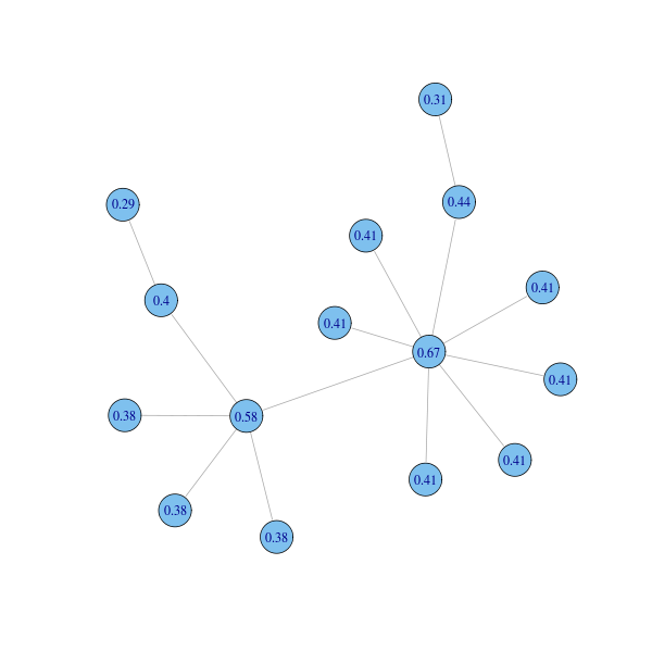
Function closeness computes closeness centrality:
clocent = closeness(g)

plot(g, layout=coords, vertex.label=round(clocent, 2))
Finally, the betweenness centrality $b_i$ of a node $i$ is the fraction of geodesic paths between other nodes that $i$ falls on:
$\displaystyle{b_i = \sum_{x, y}\frac{\sigma_{xy}(i)}{\sigma_{xy}}}$
where $x$ and $y$ and $i$ are pairwise different nodes, $\sigma_{xy}(i)$ is the number of geodesics from $x$ to $y$ that pass through $i$ and $\sigma_{xy}$ is the number of geodesics from $x$ to $y$. Betweenness is a measure of the control that a node exerts over the flow of information on the network assuming that information always takes a shortest possible path.
Betweenness centrality is computed by function betweenness. Notice that our sample graph is in fact a tree, hence the number $\sigma_{xy}$ of geodesics from $x$ to $y$ is always 1, and number $\sigma_{xy}(i)$ of geodesics from $x$ to $y$ that pass through $i$ is either 0 or 1.
btwcent = betweenness(g)

plot(g, layout=coords, vertex.label=btwcent)
Calculating closeness and betweenness centrality for all nodes in a graph involves computing the shortest paths between all pairs of nodes in the graph. If the graph has $n$ nodes and $m$ edges, this takes $O(n^3)$ time with Floyd-Warshall algorithm. On sparse graphs, Johnson algorithm is more efficient, taking $O(n^2 \log n + nm)$. Brandes devised an algorithm for unweighted graphs that requires $O(n+m)$ space and run in $O(nm)$ time.
Let's check the correlation between the four centrality measures on a random scale-free network:
g = barabasi.game(1000, m = 2, directed=FALSE, out.pref = TRUE)

degcent = degree(g)
eigcent = evcent(g)$vector
clocent = closeness(g)
btwcent = betweenness(g)

m = cbind(degcent, eigcent, clocent, btwcent)
round(cor(m), 2)

        degcent eigcent clocent btwcent
degcent    1.00    0.78    0.62    0.95
eigcent    0.78    1.00    0.76    0.85
clocent    0.62    0.76    1.00    0.58
btwcent    0.95    0.85    0.58    1.00
Not surprisingly, the four centrality measures are positively correlated. In particular, notice how nodes with a high degree have also a high betweenness centrality. Indeed, the shortest path between the neighbours of a node passes through the node unless the neighbour nodes are directly connected. Moreover, if a node $x$ has $k$ neighbours, there are $k \cdot (k-1)$ short paths of the form $u_1, x, u_2$, where $u_1$ and $u_2$ are neighbours of $x$, each of them having a good chance of being a geodesic that passes trough $x$. By contrast, degree centrality has less impact on closeness centrality. Moreover, eigenvector centrality is best associated with betweenness centrality, while closeness is the less correlated measure, in particular closeness and betweenness have the lowest correlation coefficient.
Let's see how the computed centrality measures are distributed:
par(mfcol = c(2, 2))
hist(degcent, breaks=30, main="Degree centrality", xlab="Degree")
hist(eigcent, breaks=30, main="Eigenvector centrality", xlab="Eigenvector")
hist(clocent, breaks=30, main="Closeness centrality", xlab="Closeness")
hist(btwcent, breaks=30, main="Betweenness centrality", xlab="Betweenness")
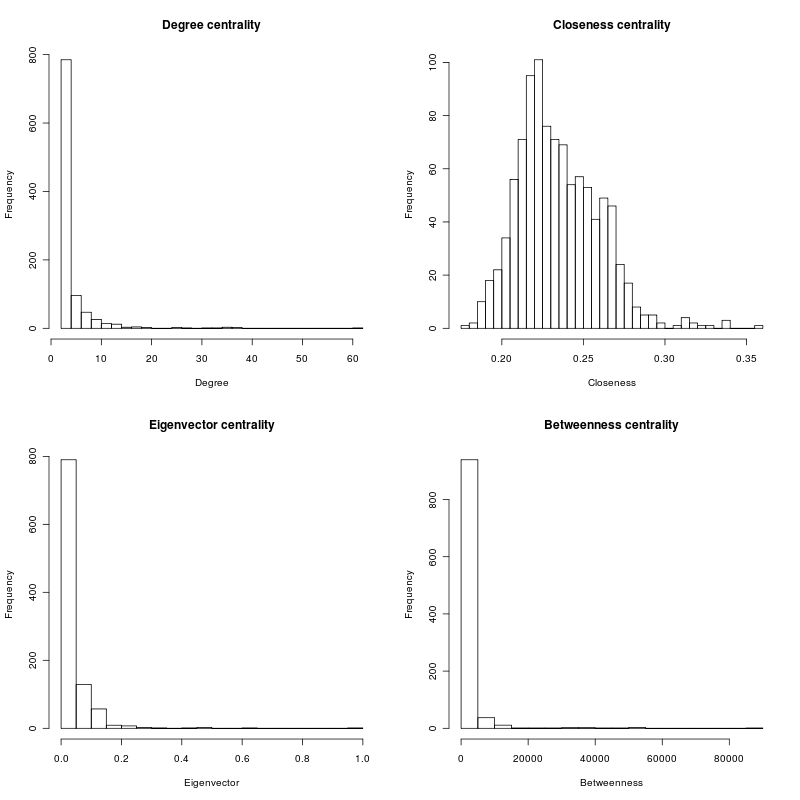
The distribution for closeness resembles a normal curve, while the other centrality measures have a long tail distribution similar to a power law.
A typical group-level analysis is network clustering. Network clustering is an organization process with the goal to put similar nodes together; the result is a partition of the network into a set of communities.
The first step in network clustering is the definition of a similarity function between nodes. In network clustering, the similarity function is typically defined in terms of the topology of the network. For instance, in an academic collaboration network, the similarity between two authors can be defined as the number of papers that the authors published together. In an article citation network, two articles are similar if they co-reference many articles or if they are co-cited many times.
When a similarity notion has been defined, we want to organize nodes into groups whose members are similar in the defined way. A cluster (or community in the network setting) is a collection of nodes which are similar between them and are dissimilar to objects belonging to other clusters. For example, communities in academic collaboration networks might represent research groups, while research topics might be the communities in citation networks.
Sometimes we know in advance the number of clusters to form. In this case, the clustering problem can be approached with partitional clustering techniques. These choose an initial partition with the decided number of clusters and then move objects between clusters trying to optimize some objective function. Examples of objective functions are the maximum distance (that is, dissimilarity) between nodes in the same cluster (to be minimized) and the minimum distance between nodes belonging to different clusters (to be maximized). The procedure stops as soon as a local stationary point for the objective function is reached. The most popular algorithm in this category is K-means.
If the size of the partition is not known in advance, then hierarchical clustering methods are more appropriate. These algorithms are of two kinds: agglomerative and divisive. An agglomerative strategy starts with a singleton partition containing a cluster for each object and then merges clusters with similar objects until the universal partition is obtained. A divisive strategy starts from the universal partition containing a unique set with all objects and then divides clusters that include dissimilar objects until the singleton partition is reached.
Both approaches can use different methods to decide what clusters to join or to divide. For instance, in agglomerative clustering, a notion of distance is defined among clusters and the two closest clusters are merged at each step. Examples of distance between two clusters are the maximum distance between elements in each cluster (complete linkage clustering), the minimum distance between elements in each cluster (single-linkage clustering), and the mean distance between elements in each cluster (average linkage clustering).
Hierarchical clustering outputs a hierarchical structure, called dendrogram, describing the whole merging/dividing process. Each horizontal cut through the dendrogram corresponds to a partition of the nodes into clusters. The dendrogram contains only a small subset of all possible partitions.
Given a set of objects, there are exponentially many partitions that can be formed. Many exact clustering problems are known to be NP-hard to solve, hence usually an approximated solution is looked for.
Network clustering techniques describes so far are an instance of data clustering methods. As an alternative approach, Rosvall and Bergstrom use ergodic random walks on networks to reveal community structure. The intuition here is as follows. Imagine a flow of information that runs across the network following the network topology. A group of nodes among which information flows quickly and easily can be aggregated and described as a single well connected module; the links between modules capture the avenues of information flow between those modules.
The authors use an infinite random walk as a proxy of the information flow and identify the modules that compose the network by minimizing the average length of the code describing a step of the random walker. This is the sum of the entropy of the movements across modules and of the entropy of movements within modules. The random walk description can be compressed if the network has regions in which the random walker tends to stay for a long time. Huffman code is exploited to encode the random walk by assigning short codewords to frequently visited nodes and modules, and longer codewords to rare ones, much as common words are short in spoken language. The minimization problem is approached using a greedy search algorithm and the solution is refined with the aid of simulated annealing. You can watch a demo at mapequaltion.org.
Despite they emerge in very different contexts, many real networks share remarkable interesting properties at the network level. Probably, the most popular feature is the small world effect. It is found that in many real webs the mean geodesic distance between node pairs is remarkably short compared to the size of the network.
The phenomenon was first told in 1929 by Hungarian poet and writer Frigyes Karinthy in a story entitled Chains, and studied in 1967 by Harvard psychologist Stanley Milgram. In a much celebrated experiment Milgram asked American people to get a postcard message to a specified target person elsewhere in the country by sending it directly to the target if the sender knew the target person on a personal basis or otherwise to a personal acquaintance who is most likely to know the target person. Milgram remarkably found that, on average, the length of the chain from the source to the target people was only six. The finding has been immortalized in popular culture in the phrase six degrees of separation.
Anecdotally, six degrees of separation is the title of a 1990 play written by John Guare and of the following movie directed by Fred Schepisi that was adapted from the play. Both were inspired by the small world phenomenon. The enchanting Alejandro González Iñárritu Oscar-winning film Babel is based on the same concept: the lives of all of the characters are dramatically intertwined, although they do not know each other and live in different continents.
While the average geodesic distance between pairs of nodes in the graph is usually small, the largest geodesic distance, called the diameter of the network, can be large.
Another interesting property shared by many real networks is clustering, also known as transitivity. In common parlance, this means that the friend of my friend is also my friend. Given a connected triple $x$, $y$ and $z$ such that $x$ is linked to both $y$ and $z$, an interesting question is: what is the probability that $y$ and $z$ are also connected forming a triangle? In particular, is this probability higher than for randomly chosen nodes?
In most real-world networks, the probability of transitively closing a connected triple into a triangle is significantly high. The clustering coefficient of a network measures this probability and can be defined as:
$\displaystyle{C = 3 \frac{N_\bigtriangleup}{N_\wedge}}$
where $N_\bigtriangleup$ is the number of triangles and $N_\wedge$ is the number of connected triples in the network. The factor 3 constrains the coefficient to lie in the range between 0 and 1.
In a much influential sociology paper, The Strength of Weak Ties, Mark Granovetter analysed the social network of people acquaintances and found that our society is far from a random world. It is structured into strongly connected clusters with few external weak ties connecting these cliques. These weak ties are in fact very strong: they play a crucial role in our ability to communicate outside of our close-knit circle of friends.
Most real instances of networks exhibit a giant component and many much smaller components. This is a large group of connected nodes of the graph occupying a sizable fraction of the whole network. The size of the giant component is propositional to the size of the graph. By contrast, the other connected components of the graph are much smaller, usually of logarithmic size with respect to the network largeness.
Finally, real networks possess a node degree distribution with a heavy tail that resembles a power law. This means that the probability $P(k)$ that a node has $k$ neighbours is roughly $k^{-\alpha}$, where $\alpha$ is a parameter that usually lies between 2 and 3. It follows that for most real webs the Pareto principle applies to node degrees: the overwhelming majority of nodes have low degrees while a few hubs possess an extraordinary number of neighbours. For instance, the majority of papers published in a journal collect a low share of citations, while there are few citational blockbusters that harvest the majority of citations.
The corresponding webs are called scale-free networks, meaning that there exists no node with a degree that is characteristic for all nodes in the network. Putting it another way, the degree distribution is highly skewed to the right and hence the distribution mean is not a good indicator of central tendency as it is for normal bell-shaped distributions.
These properties of real networks can be exploited in two perspectives: on the one hand, they are useful to understand how these networks emerged. A number of models of network growth have been proposed to explain the generation of networks with similar properties. On the other hand, knowing the topological properties of real networks is crucial to study the processes taking place on networks, like the propagation of information or any other quantity on the network.