The excellent book Google's PageRank and Beyond of Amy N. Langville and Carl D. Meyer elegantly describes the science of search engine rankings in a rigorous yet playful style. In the following, we briefly recall how the PageRank method works.
Before giving the mathematical formulation of the problem solved by the PageRank method, we provide an intuitive interpretation of PageRank in terms of random walks on graphs. The Web is viewed as a directed graph of pages connected by hyperlinks. A random surfer starts from an arbitrary page and simply keeps clicking on successive links at random, bouncing from page to page. The PageRank value of a page corresponds to the relative frequency the random surfer visits that page, assuming that the surfer goes on infinitely. The higher is the number of times the random surfer visits a page, the higher is the status, measured in terms of PageRank, of the page.
In mathematical terms, the method can be described as follows. Let us denote by $q_i$ the number of forward (outgoing) links of page $i$. Let $H = (h_{i,j})$ be a square transition matrix such that $h_{i,j} = 1 / q_i$ if there exists a link from page $i$ to page $j$ and $h_{i,j} = 0$ otherwise. Page self-links are ignored, hence $h_{i,i} = 0$ for all $i$. The value $h_{i,j}$ can be interpreted as the probability that the random surfer moves from page $i$ to page $j$ by clicking on one of the hyperlinks of page $i$. The PageRank $\pi_j$ of page $j$ is recursively defined as:
$\displaystyle{\pi_j = \sum_i \pi_i h_{i,j}}$
or, in matrix notation:
$\displaystyle{\pi = \pi H}$
Hence, the PageRank of page $j$ is the sum of the PageRank scores of pages $i$ linking to $j$, weighted by the probability of going from $i$ to $j$.
Unfortunately, the described ideal model has two problems that prevent the solution of the system. The first one is due to the presence of dangling nodes, that are pages with no forward links. These pages capture the random surfer indefinitely. Notice that a dangling node corresponds to a row in $H$ with all entries equal to 0. To tackle the problem, such rows are replaced by a bookmark vector $b$ such that $b_i > 0$ for all $i$ and $\sum_i b_i = 1$. This means that the random surfer escapes from the dangling page by jumping to a completely unrelated page according to the bookmark probability distribution. Let $S$ be the resulting matrix.
The second problem with the ideal model is that the surfer can get trapped by a closed cycle in the Web graph, for instance, two pages A and B such that A links only to B and B links only to A. The solution proposed by Brin and Page is to replace matrix $S$ by Google matrix:
$\displaystyle{G = \alpha S + (1-\alpha) T}$
where $T$ is the teleportation matrix with identical rows each equal to the bookmark vector $b$, and $\alpha$ is a free balancing parameter of the algorithm. The interpretation is that, with probability $\alpha$ the random surfer moves forward by following links, and, with the complementary probability $1 - \alpha$ the surfer gets bored of following links and it is teleported to a random page chosen in accordance with the bookmark distribution. The inventors of PageRank propose to set $\alpha = 0.85$, meaning that after about five link clicks the random surfer chooses from bookmarks. The PageRank vector is then defined as the solution of equation:
$\displaystyle{\pi = \pi G}$

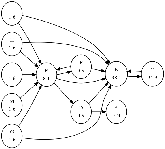
Figure above shows a PageRank instance with solution. Each node is labelled with its PageRank score; scores have been normalized to sum to 100 and are approximated to the first decimal point. We assumed $\alpha = 0.85$ and each bookmark probability equal to $1/n$, where $n = 11$ is the number of nodes. Node A is a dangling node, and nodes B and C form a dangling cycle. Notice the dynamics of the method: node C receives just one link but from the most important page B, hence its importance is higher than that of E, which receives much more links (5) but from anonymous pages. Pages G, H, I, L, and M do not receive endorsements; their scores correspond to the minimum amount of status assigned to each page.
We can use the iterative Power Method on $G$ to compute the PageRank vector as follows:
$\displaystyle{ \begin{array}{lcl} \pi_0 & = & e/n \\ \pi_{k+1} & = & \pi_{k} G \end{array} }$where $e$ is a vector of 1's. Furthermore, notice that the adjacency matrix $H$ is typically a sparse matrix, but $G$ is a dense matrix. We can apply the Power Method directly to $H$ as follows. Let $a$ be a dangling vector such as $a_i = 1$ if $i$ is a dangling node and $a_i = 0$ otherwise. With a little algebra we have that:
$\displaystyle{ \begin{array}{lcl} G & = & \alpha S + (1-\alpha) T \\ & = & \alpha (H + a b^T) + (1-\alpha) e b^T \\ & = & \alpha H + (\alpha a + (1-\alpha) e) b^T \end{array} }$
Hence, the Power Method becomes:
$\displaystyle{ \begin{array}{lcl} \pi_0 & = & e/n \\ \pi_{k+1} & = & \alpha \pi_{k} H + (\alpha \pi_{k} a + (1-\alpha) \pi_{k} e) b^T \end{array} }$
Let's do all this in R:
# EXACT SMALL-SCALE COMPUTATION OF PAGERANK
# H = adjacency matrix
# b = bookmark vector
# alpha = balancing parameter

exact.pr = function (H, b, alpha = 0.85) {

  n = dim(H)[1]
  # normalize adjacency matrix by row sum and
  # replace dangling rows with bookmark vector (S matrix)
  S = H
  # compute row sums
  rs = H %*% rep(1,n)
  for (i in 1:n) {
    if (rs[i] == 0) {
      S[i,] = b
    } else {
      S[i,] = S[i,] / rs[i]
    }
  }

  # build teleportation matrix
  T = rep(1, n) %*% t(b)

  # build Google matrix
  G = alpha * S + (1-alpha) * T

  # compute eigenpairs and retrieve the leading eigenvector
  eig = eigen(t(G))
  pi = as.real(eig$vectors[,1])
  pi = pi / sum(pi)
  return(pi)
}

# APPROXIMATED SMALL-SCALE COMPUTATION OF PAGERANK (uses dense matrix G)
# H = adjacency matrix
# b = bookmark vector
# alpha = balancing parameter
# t = number of digits of precision

approx.pr = function (H, b, alpha = 0.85, t = 3) {

  n = dim(H)[1]
  # normalize adjacency matrix by row sum and
  # replace dangling rows with bookmark vector (S matrix)
  S = H
  # compute row sums
  rs = H %*% rep(1,n)
  for (i in 1:n) {
    if (rs[i] == 0) {
      S[i,] = b
    } else {
      S[i,] = S[i,] / rs[i]
    }
  }


  # build teleportation matrix
  T = rep(1, n) %*% t(b)

  # build Google matrix
  G = alpha * S + (1-alpha) * T

  pi0 = rep(0, n)
  pi1 = rep(1/n, n)
  eps = 1/10^t
  iter = 0
  while (sum(abs(pi0 - pi1)) > eps) {
    pi0 = pi1
    pi1 = pi1 %*% G
    iter = iter + 1
  }
  pi1 = pi1 / sum(pi1)
  return(list(pi = pi1, iter = iter))
}

# APPROXIMATED LARGE-SCALE COMPUTATION OF PAGERANK (uses sparse matrix H)
# H = adjacency matrix
# b = bookmark vector
# alpha = balancing parameter
# t = number of digits of precision

approx.fast.pr = function (H, b, alpha = 0.85, t = 3) {

  n = dim(H)[1]
  # normalize adjacency matrix by row sum and compute dangling node vector
  a = rep(0, n)
  # compute row sums
  rs = H %*% rep(1,n)
  for (i in 1:n) {
    if (rs[i] == 0) {
      a[i] = 1
    } else {
      H[i,] = H[i,] / rs[i]
    }
  }

  e = rep(1, n)
  pi0 = rep(0, n)
  pi1 = rep(1/n, n)
  eps = 1/10^t
  iter = 0
  while (sum(abs(pi0 - pi1)) > eps) {
    pi0 = pi1
    pi1 = alpha * pi1 %*% H + (alpha * pi1 %*% a + (1 - alpha) * pi1 %*% e) * b
    iter = iter + 1
  }
  pi1 = pi1 / sum(pi1)
  return(list(pi = pi1, iter = iter))
}
We first try with the toy example depicted in the above graph:
n = 11
H = matrix(scan("pagerank.txt",0), nrow=n, byrow=TRUE)
b = rep(1/n, n)
alpha = 0.85
t = 10

> exact.pr(H, b, alpha)
 [1] 0.03278149 0.38440095 0.34291029 0.03908709 0.08088569 0.03908709
 [7] 0.01616948 0.01616948 0.01616948 0.01616948 0.01616948

> approx.pr(H, b, alpha, t)
$pi
           [,1]      [,2]      [,3]       [,4]      [,5]       [,6]       [,7]
[1,] 0.03278149 0.3844009 0.3429103 0.03908709 0.0808857 0.03908709 0.01616948
           [,8]       [,9]      [,10]      [,11]
[1,] 0.01616948 0.01616948 0.01616948 0.01616948

$iter
[1] 137

> approx.fast.pr(H, b, alpha, t)
$pi
           [,1]      [,2]      [,3]       [,4]      [,5]       [,6]       [,7]
[1,] 0.03278149 0.3844009 0.3429103 0.03908709 0.0808857 0.03908709 0.01616948
           [,8]       [,9]      [,10]      [,11]
[1,] 0.01616948 0.01616948 0.01616948 0.01616948

$iter
[1] 137
In the following we generate random graphs and use them to benchmark the different PageRank computation methods:
# COMPUTE A RANDOM DIRECTED GRAPH
# n = number of nodes
# p = outlink probability (each node will have p * n successors on average)

randG = function(n, p) {
  adj =  matrix(nrow=n, ncol=n)
  for (i in 1:n) {
    adj[i,] = sample(c(0,1), n, replace=TRUE, prob=c(1-p, p))
  }
  return(adj)
}

n = 1000;
p = 0.1;
H = randG(n, p)
b = rep(1/n, n)
alpha = 0.85
t = 10

> system.time(exact.pr(H, b, alpha))
   user  system elapsed
 62.424   0.932 101.097

> system.time(approx.pr(H, b, alpha, t))
   user  system elapsed
  1.372   0.036   1.408

> system.time(approx.fast.pr(H, b, alpha, t))
   user  system elapsed
  0.904   0.000   0.904
The performance of approx.fast.pr can be significantly enhanced using a sparse representation for matrix $H$.
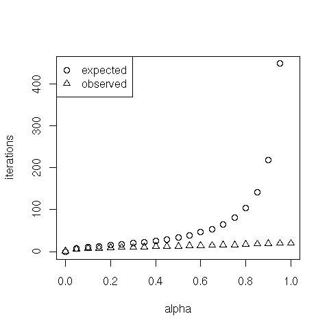
Let's test how the balancing parameter $\alpha$ influences the computational speed (number of iterations) of the approximated methods:
n = 100;
p = 0.1;
H = randG(n, p)
b = rep(1/n, n)
aseq = seq(0, 1, 0.05)
t = 10
i = 1
iter = NULL
for (alpha in aseq) {
  iter[i] = approx.fast.pr(H, b, alpha, t)$iter
  i = i + 1
}

names(iter) = aseq

> iter
   0 0.05  0.1 0.15  0.2 0.25  0.3 0.35  0.4 0.45  0.5 0.55  0.6 0.65  0.7 0.75
   1    6    7    8    9   10   10   11   12   12   13   14   14   15   16   16
 0.8 0.85  0.9 0.95    1
  17   18   19   20   20

plot(aseq, iter, xlab="alpha", ylab="iterations")
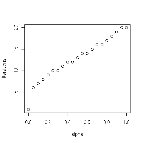
The asymptotic rate of convergence of the power method depends on the ratio of the two eigenvalues of $G$ that are largest in magnitude, denoted $\lambda_1$ and $\lambda_2$. Specifically, it is the rate at which $|\lambda_2 / \lambda_1|^k$ goes to 0. Since $G$ is stochastic, $\lambda_1 = 1$, so $|\lambda_2|$ governs the convergence. It turns out that $\lambda_2 = \alpha \mu_2$, where $\mu_2$ is the subdominant eigenvalue of $S$. It is expected that, for matrices representing the link structure of the Web, $\mu_2$ is close to 1, so the convergence rate is $\alpha^k$. Hence, to produce scores with $\tau$ digits of precision we must have $10^{-\tau} = \alpha^k$ and thus about $k = -\tau / \log_{10} \alpha$ iterations must be completed. Is the observed computation faster than expected?
exp.iter = ceiling(-t / log10(aseq))
names(exp.iter) = aseq

> exp.iter
   0 0.05  0.1 0.15  0.2 0.25  0.3 0.35  0.4 0.45  0.5 0.55  0.6 0.65  0.7 0.75
   0    8   10   13   15   17   20   22   26   29   34   39   46   54   65   81
 0.8 0.85  0.9 0.95    1
 104  142  219  449 -Inf

> iter
   0 0.05  0.1 0.15  0.2 0.25  0.3 0.35  0.4 0.45  0.5 0.55  0.6 0.65  0.7 0.75
   1    6    7    8    9   10   10   11   12   12   13   14   14   15   16   16
 0.8 0.85  0.9 0.95    1
  17   18   19   20   20

plot(aseq, exp.iter, xlab="alpha", ylab="iterations")
points(aseq, iter, pch=2)
legend(x = "topleft", legend = c("expected", "observed"), pch = c(1,2))
Why so fast? Let's check the dominant and subdominant eigenvalues of matrices $S$ and $G$:
alpha = 0.85
S = H
rs = H %*% rep(1,n)
for (i in 1:n) {
  if (rs[i] == 0) {
    S[i,] = b
  } else {
    S[i,] = S[i,] / rs[i]
  }
}

T = rep(1, n) %*% t(b)
G = alpha * S + (1-alpha) * T

val.S = eigen(S)$val
val.G = eigen(G)$val

> abs(val.S[1:2])
[1] 1.0000000 0.3322384

> abs(val.G[1:2])
[1] 1.0000000 0.2824027

> abs(val.S[2]) * alpha
[1] 0.2824027
Notice that the subdominant eigenvalue of $S$ is far from 1, and this speeds up the computation. In fact, the generated matrix $H$ is a random graph, and not a scale-free network as the link structure of the Web. Let us simulate the Web graph with scale-free networks:
# Pareto distribution
dpareto=function(x, shape=1, location=1) shape*location^shape/x^(shape+1);
ppareto=function(x, shape=1, location=1) (x >= location)*(1-(location/x)^shape);
qpareto=function(u, shape=1, location=1) location/(1-u)^(1/shape);
rpareto=function(n, shape=1, location=1) qpareto(runif(n),shape,location);

# GENERATE A SCALE-FREE DIRECTED GRAPH
# n = number of nodes
# shape = the exponent parameter of power law
# location = the min value parameter of power law

paretoG = function(n, shape=1, location=1) {
  degree = round(rpareto(n, shape, location))
  degree[degree > n] = n
  adj =  matrix(0, nrow=n, ncol=n)
  for (i in 1:n) {
    index = sample(1:n, degree[i])
    adj[i, index] = 1
  }
  return(adj)
}
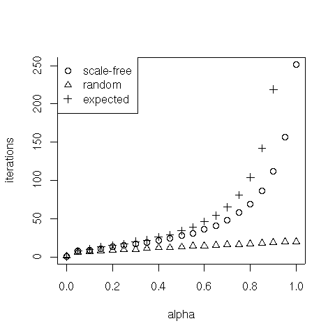
In the following we test the how $\alpha$ influences the number of iterations on scale-free graphs:
n = 100
shape = 1.5
location = 1
sf.H = paretoG(n, shape, location)
b = rep(1/n, n)
aseq = seq(0, 1, 0.05)
t = 10
i = 1
sf.iter = NULL
for (a in aseq) {
  sf.iter[i] = approx.fast.pr(sf.H, b, a, t)$iter
  i = i + 1
}
names(sf.iter) = aseq

> sf.iter
   0 0.05  0.1 0.15  0.2 0.25  0.3 0.35  0.4 0.45  0.5 0.55  0.6 0.65  0.7 0.75
   1    8    9   11   13   15   17   19   22   24   28   31   36   41   48   58
 0.8 0.85  0.9 0.95    1
  69   86  112  157  251

> exp.iter
   0 0.05  0.1 0.15  0.2 0.25  0.3 0.35  0.4 0.45  0.5 0.55  0.6 0.65  0.7 0.75
   0    8   10   13   15   17   20   22   26   29   34   39   46   54   65   81
 0.8 0.85  0.9 0.95    1
 104  142  219  449 -Inf

> iter
   0 0.05  0.1 0.15  0.2 0.25  0.3 0.35  0.4 0.45  0.5 0.55  0.6 0.65  0.7 0.75
   1    6    7    8    9   10   10   11   12   12   13   14   14   15   16   16
 0.8 0.85  0.9 0.95    1
  17   18   19   20   20

plot(aseq, exp.iter, xlab="alpha", ylab="iterations")
points(aseq, sf.iter, pch=2)
points(aseq, iter, pch=3)
legend(x = "topleft", legend = c("expected", "scale-free", "random"), pch = c(1, 2, 3))
Let's check the subdominant eigenvalues of $S$:
S = sf.H
rs = sf.H %*% rep(1,n)
for (i in 1:n) {
  if (rs[i] == 0) {
    S[i,] = b
  } else {
    S[i,] = S[i,] / rs[i]
  }
}
val.S = eigen(S)$val

> abs(val.S[2])
[1] 0.9194817
Notice that the subdominant eigenvalue of $S$ is now much closer to 1. This explains why the convergence rate is slower than what observed on random networks.
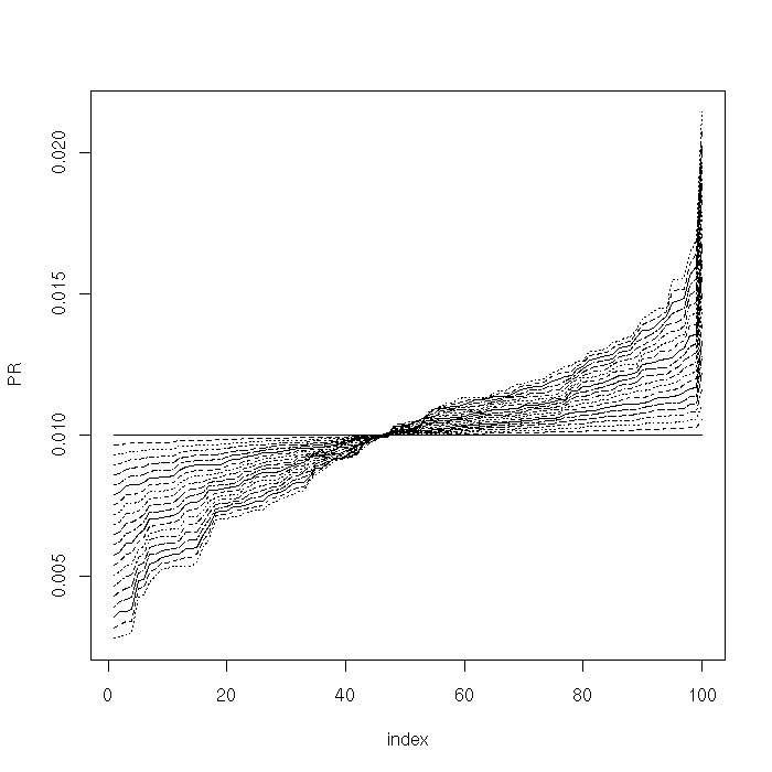
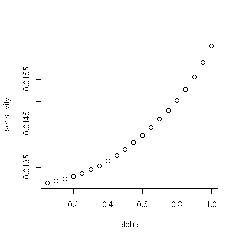
We now check the sensitivity of the PageRank vector to variations of the balancing parameter $\alpha$. From theory, we know that, for small $\alpha$, PageRank is insensitive to slight variations in $\alpha$. As $\alpha$ becomes larger, PageRank becomes increasingly more sensitive to small perturbations in $\alpha$.
n = 100;
p = 0.1;
H = randG(n, p)
b = rep(1/n, n)
aseq = seq(0, 1, 0.05)
t = 10
i = 1
Pi = matrix(nrow = length(aseq), ncol = n)
for (a in aseq) {
  Pi[i,] = approx.fast.pr(H, b, a, t)$pi
  i = i + 1
}
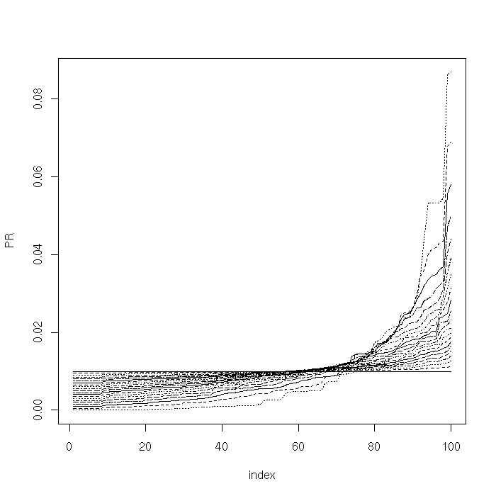
We plot the PageRank vectors for different values of $\alpha$:
plot(sort(Pi[1,]), type = "l", lty = 1, xlab="index", ylab="PR", ylim = c(min(Pi), max(Pi)))
for (i in 2:length(aseq)) {
  lines(sort(Pi[i,]), lty = i)
}
We furthermore compute and plot (norm 1) distance between PageRank vectors for different values of $\alpha$:
d = NULL
for (i in 2:length(aseq)) {
  d[i-1] = sum(abs(Pi[i,] - Pi[i-1,]))
}
plot(aseq[2:length(aseq)], d, xlab="alpha", ylab="sensitivity")
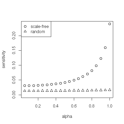
For $\alpha$ close to 1, the degree of sensitivity is governed (again) by the subdominant eigenvalue of $S$. Hence we might expect higher sensitivity on scale-free graphs. Let's check it:
n = 100
shape = 1.5
location = 1
sf.H = paretoG(n, shape, location)
b = rep(1/n, n)
aseq = seq(0, 1, 0.05)
t = 10
i = 1
Pi = matrix(nrow = length(aseq), ncol = n)
for (a in aseq) {
  Pi[i,] = approx.fast.pr(sf.H, b, a, t)$pi
  i = i + 1
}

plot(sort(Pi[1,]), type = "l", lty = 1, xlab="index", ylab="PR", ylim = c(min(Pi), max(Pi)))
for (i in 2:length(aseq)) {
  lines(sort(Pi[i,]), lty = i)
}

sf.d = NULL
for (i in 2:length(aseq)) {
  sf.d[i-1] = sum(abs(Pi[i,] - Pi[i-1,]))
}

plot(aseq[2:length(aseq)], sf.d, xlab="alpha", ylab="sensitivity", ylim=c(0, max(sf.d)))
points(aseq[2:length(aseq)], d, pch=2)
legend(x = "topleft", legend = c("scale-free", "random"), pch = c(1, 2))
