This method is similar to Kleinberg centrality. Like Kleinberg centrality, offense-defense method assigns to each node two scores: an offensive rating and a defensive rating. Unlike Kleinberg measure, in offense-defense method the relationships between the two scores is non-linear. The offense-defense power thesis reads:
A node has high offensive rating if it is linked to by nodes with low defensive rating; a node has high defensive rating if it links to nodes with low offensive rating.
The method is described in Amy N. Langville and Carl D. Meyer's book Who's #1? (The Science of Rating and Ranking). In the book the method is applied to the problem of rating and ranking of sport teams; however, it can be tailored for different contexts, for instance financial networks in which offense is credit and defense is debit. In this section we follow the convenient presentation of the book of Langville and Meyer. In sport, the offensive strength of team A during a match with team B is a relative concept since it depends on the defensive prowess of team B: winning against a team with a strong defense significantly increases the offensive power of the winner; similarly, the defensive power of team A is relative to the offensive skill of team B: losing against a team with a weak offense significantly deflates the defensive power of the loser.
Let $A = (a_{i,j})$ be the adjacency matrix of a weighted directed graph. We interpret $a_{i,j}$ as the score that team $j$ generated against team $i$ (average the results if the teams met more than once). Set $a_{i,j} = 0$ if the two teams did not play each other. Notice that $a_{i,j}$ reflects both offensive and defensive strength: it is the number of points that $j$ scores to $i$ (an offensive indicator) as well as the number of points that $i$ held $j$ to (a defensive indicator).
Offensive rating $x_{i}$ of team $i$ is given by: $$x_i = \sum_k \frac{a_{k,i}}{y_k}$$ and defensive rating $y_{i}$ of team $i$ is given by: $$y_i = \sum_k \frac{a_{i,k}}{x_k}$$ Observe that large offensive rating corresponds to strong offense; on the other hand large defensive rating corresponds to weak defense. Hence, one can define offensive power as offensive rating $x_i$, and defensive power as the reciprocal of defensive rating $1/y_i$: teams with high offensive power, are those that scores many points against teams with large defensive power; teams with high defensive power are those that gets few points against teams with large offensive power.
Let $x^{\div} = 1/x$ be the vector whose elements are the reciprocals of the elements of $x$. In matrix form we have: $$\begin{array}{lcl} x & = & y^{\div} A\\ y & = & x^{\div} A^T \\ \end{array}$$ or, combining the two: $$\begin{array}{lcl} x & = & (x^{\div} A^T)^{\div} A \\ y & = & (y^{\div} A)^{\div} A^T \\ \end{array}$$
Notice that in the offense-defense power the relationships between the two measures is non-linear, while in Kleinberg centrality this relationships is linear. Hence, offense-defense method can be regarded as a non-linear (reciprocal) version of Kleinberg method.
A single offense-defense rating for a team can be obtained by combining the offense and defense ratings as follows: $$z_i = \frac{x_i}{y_i}$$ A team $i$ with high offense-defense power $z_i$ has a large offensive power $x_i$ as well as a large defensive power $1/y_i$: it is strong in both offense and defense.
Offense and defense ratings can be computed with the following iterative process. Let $y_0 = e$, where $e$ is the vector of all 1's. For $k \geq 1$: $$\begin{array}{lcl} x_k & = & y_{k-1}^{\div} A\\ y_k & = & x_{k}^{\div} A^T \\ \end{array}$$ or alternatively, setting $x_0 = y_0 = e$: $$\begin{array}{lcl} x_k & = & (x_{k-1}^{\div} A^T)^{\div} A \\ y_k & = & (y_{k-1}^{\div} A)^{\div} A^T \\ \end{array}$$ For instance, the first-iteration offense is $(e A^T)^{\div} A$; for a given node $i$ it is the sum of reciprocals of out-degrees (points conceded) of predecessors of $i$ (teams against which $i$ has scored). The first-iteration defense is $(e A)^{\div} A^T$; for a given node $i$ it is the sum of reciprocals of in-degrees (points scored) of successors of $i$ (teams that scored against $i$). There is in fact no need to use both of these iterations because if we can produce the ratings from one of them, the other ratings are obtained from $x = y^{\div} A$ and $y = x^{\div} A^T$.
By Sinkhorn-Knopp theorem, the offensive and defensive powers exist, and the corresponding iterative method converges, if and only if the corresponding graph $G_A$ is regularizable. What about the offense defense method on graphs that are not regularizable? A solution is recaptured using a perturbed matrix $$A_\epsilon = A + \epsilon E$$ where $\epsilon > 0$ and $E$ is a matrix full of 1's. Notice that $A_\epsilon > 0$ and hence the graph of $A_\epsilon$ is complete (it has all possible edges), thus it is regular and regularizable. Moreover, if $\epsilon$ is small relative to the nonzero entries in the original matrix, then the spirit of the original data is not overly compromised. However, the smaller $\epsilon$, the larger the number of iterations needed to produce viable results. In other words, the choice of $\epsilon$ is a compromise between quality and efficiency of the solution.
The following user-defined function od computes offense and defense ratings using a direct computation:
# Compute offense x = (1/y) A and defense y = A (1/x)
#INPUT
# A = graph adjacency matrix
# t = precision
# OUTPUT
# A list with:
# x = offense vector
# y = defense vector
# iter = number of iterations
od = function(A, t) {
  n = dim(A)[1];
  y0 = rep(1, n);
  diff = 1
  eps = 1/10^t;
  iter = 0;
  while (diff > eps) {
    x1 = (1/y0) %*% A;
    y1 = (1/x1) %*% t(A);
    diff = sum(abs(y1 - y0));
    y0 = y1;
    iter = iter + 1;
  }
  return(list(o = as.vector(x1), d = as.vector(y1), iter = iter))
}
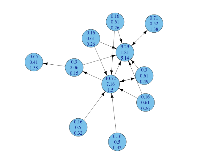
A directed graph with nodes labelled with the following ratings from top to bottom: offensive, defensive, and aggregated. The graph is not regularizable, hence the full perturbation has been used. Notice how the two central nodes have both large offensive power, but only one has also a large defensive power (a small defensive rating): this is the node with the largest aggregated offense-defense power.