Typically, geodesic (shortest) paths are considered in the definition of both closeness and betweenness. These are optimal paths with the lowest number of edges or, if the graph is weighted, paths with the smallest sum of edge weights. There are two drawbacks of this approach:
In many applications, however, it is reasonable to consider the abundance and the length of all paths of the network, since communication on the network is enhanced as soon as more routes are possible, in particular if these pathways are short. Hence, we look for a distance measure among nodes such that nodes separated by many short paths are close, while nodes separated by few long paths are far away.
A solution comes from electromagnetism. Recall that Ohm's law says $$I = \frac{V}{R} = V C$$ where $V$ is the potential difference, $I$ the current intensity, $R$ the resistance and $C = 1/R$ is the conductance. The effective resistance of series and parallel circuits can be computed as follows:
Hence, effective resistance has the properties we are looking for, that is it is directly influenced by the length and abundance of paths between two nodes.
More generally, consider a connected undirected network in which each edge is assigned with a positive weight corresponding to the strength of the relationship between the nodes linked by the edge. The edges are viewed as resistors and the nodes as junctions between resistors. The edge weight is the conductance (the reciprocal of resistance) of the edge. Outlets are particular nodes where current enters and leaves the network. This is called resistor network. Our goal is to compute the effective resistance between any two nodes in this general setting and use it to define closeness and betweenness notions that take into considerations all paths (with different weights).
Let's work out the mathematical details. A vector $u$ called supply defines outlets: a node $i$ such that $u_i \neq 0$ is an outlet; in particular if $u_i > 0$ then node $i$ is a source and current enters the network through it, while if $u_i < 0$ then node $i$ is a target and current leaves the network through it. Since there should be as much current entering the network as leaving it, we have that $\sum_i u_i = 0$. We consider the case where a unit of current enters the network at a single source $s$ and leaves it at a single target $t$. That is, $u_{i}^{(s,t)} = 0$ for $i \neq s,t$, $u_{s}^{(s,t)} = 1$, and $u_{t}^{(s,t)} = -1$. Let $v_{i}^{(s,t)}$ be the potential of node $i$, measured relative to any convenient reference potential, for source $s$ and target $t$ outlets. Kirchhoff's law of current conservation implies that the node potentials satisfy the following equation for every node $i$:
$$\sum_j A_{i,j} (v_{i}^{(s,t)} - v_{j}^{(s,t)}) = u_{i}^{(s,t)}$$where $A$ is the weighted adjacency matrix of the network. By Ohm's law, the current flow through edge $(i,j)$ is the quantity $A_{i,j} (v_{i}^{(s,t)} - v_{j}^{(s,t)})$, that is, the difference of potentials between the involved nodes multiplied by the conductance of the edge: a positive value indicates that the current flows in a direction (say from $i$ to $j$), and negative value means that the current flows in the opposite direction. Hence, Krichhoff's law states that the current flowing in or out of any node is zero, with the exception of the source and target nodes. In matrix form, Kirchhoff law reads:
$$(D-A) v^{(s,t)} = Gv^{(s,t)} = u^{(s,t)}$$where $D$ is a diagonal matrix such that the $i$-th element of the diagonal is equal to $\sum_j A_{i,j}$, that is, it is the (weighted) degree of node $i$. The matrix $G = D-A$ is called the graph Laplacian.
Notice that all rows of $G$ sum to 0, that is, $G e = 0$, where $e$ is a vector with all elements equal to 1. Hence 0 is an eigenvalue of $G$ corresponding to the eigenvector $e$, thus the determinant of $G$ is 0 and hence $G$ is not invertible. Nevertheless, the linear system $$Gv^{(s,t)} = u^{(s,t)}$$ has a solution, in fact it has infinite many solutions: if $v^*$ is a solution, then, for any scalar $\alpha$, it holds that $v^* + \alpha$ is also a solution. Hence, any two solutions differ by a constant. This is because all rows of the Laplacian matrix $G$ sum to zero. A solution for the equation $Gv^{(s,t)} = u^{(s,t)}$ is given by the Moore-Penrose generalized inverse $G^+$ of $G$:
$$v^{(s,t)} = G^+ u^{(s,t)}$$that is:
$$v_{i}^{(s,t)} = G_{i,s}^{+} - G_{i,t}^{+}$$where the generalized inverse $G^+$ is obtained from $G$ as follows:
$$G^+=(G+ee^T/n)^{-1}-ee^T/n$$Therefore, the generalized inverse matrix $G^+$ contains information to compute all node potentials for any pair of source-target nodes. Notice, however, that $G + ee^T/n$ is a full matrix, even if the graph of $A$ is sparse. Hence, inverting it might be computationally heavy.
A solution for the equation $Gv^{(s,t)} = u^{(s,t)}$ can be also obtained as follows. Get the reduced Laplacian matrix $G'$ by removing the i-th row and column, for any fixed $i$. Invert matrix $G'$. Notice that $G'$ is sparse if the graph of $A$ is sparse. Finally, add back to the inverted matrix an i-th row and column made of all 0s. Let $G^-$ be the resulting matrix, that we call inverted reduced Laplacian. Now, compute $$v^{(s,t)} = G^- u^{(s,t)}.$$ The solution obtained with the reduced Laplacian $G^-$ differs from the one obtained using the generalized inverse $G^+$ by a constant. This will be no problem, since in general we are not interested in the absolute value of the potential for a point, but instead in the potential difference between two points.
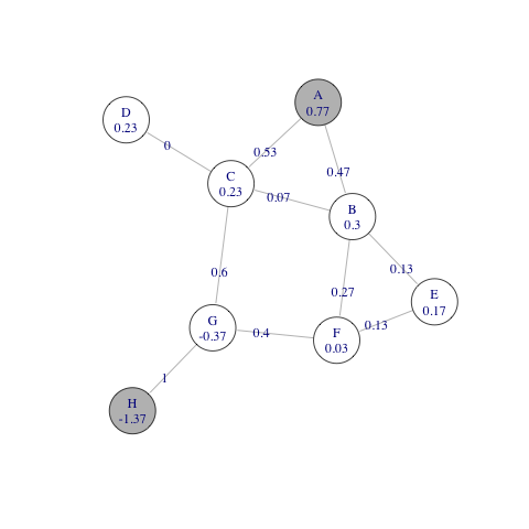
The following figure depicts a resistor network with all resistances equal to unity. Each node is identified with a letter and is labelled with the value of its potential when a unit current is injected in node A and removed from node H. Each edge is labelled with the absolute current flowing on it (the absolute potential difference between the nodes of the edge). Notice that Kirchhoff's law is satisfied for each node. For instance, the current entering in node B is 0.47 (from node A) which equals the current leaving node B, which is again 0.47 (0.13 to E, 0.27 to F, and 0.07 to C). Moreover, the current leaving the source node A is 1, and the current entering the target node H is also 1. Notice that there is no current on the edge from C to D, since both nodes have the same potential.
We are now ready to define the effective resistance between two nodes in a resistor network and define it as a distance. Given nodes $i$ and $j$, the resistance distance $R_{i,j}$ between $i$ and $j$ is the effective resistance between $i$ and $j$ when a unit of current is injected from source $i$ and removed from target $j$. Since the current is unity, this is also the potential difference of nodes $i$ and $j$:
$$R_{i,j} = v_{i}^{(i,j)} - v_{j}^{(i,j)} = (G_{i,i}^{+} - G_{i,j}^{+}) - (G_{j,i}^{+} - G_{j,j}^{+}) = G_{i,i}^{+} + G_{j,j}^{+} - 2 G_{i,j}^{+}$$(notice that $G$ and $G^+$ are both symmetric). In matrix form, we have that: $$R = e \, diag(G^+)^T + diag(G^+)e^T - 2G^+,$$ where $e$ is a vector with all components equal to 1, and $diag(G^+)$ is the diagonal of matrix $G^+$. Equivalently, we can define $R$ in terms of the inverted reduced Laplacian $G^-$: $$R = e \, diag(G^-)^T + diag(G^-)e^T - 2G^-$$ In fact the resistance distance is a metric on the graph: $R_{i,j} > 0$ if $i \neq j$ and $R_{i,i} = 0$; $R_{i,j} = R_{j,i}$, and $R_{i,j} \leq R_{i,k} + R_{k,j}$. For instance, the resistance distance between A and H in the above graph is 2.14. Notice that this is smaller than the shortest-path distance between A and H, which is 3, since there are multiple paths connecting the two nodes.
Current-flow closeness centrality uses the notion of resistance distance. Hence, given two nodes $i$ and $j$, the distance between them is the resistance distance $R_{i,j}$. The mean distance $d_i$ of node $i$ from the other nodes is then defined by:
$\displaystyle{d_{i} = \frac{\sum_{j} R_{i,j}}{n}}$
and current-flow closeness centrality for node $i$ is:
$\displaystyle{c_i = \frac{1}{d_i} = \frac{n}{\sum_{j} R_{i,j}}}$
We next give the precise definition of current-flow betweenness centrality. The idea is that the betweenness of a node with respect to a pair of source and target nodes is proportional to the amount of current that flows though the node when a unit of current is injected at the source node and removed at the target node. As observed above, given a source $s$ and a target $t$, the absolute current flow through edge $(i,j)$ is the quantity $A_{i,j} |v_{i}^{(s,t)} - v_{j}^{(s,t)}|$. By Kirchhoff's law the current that enters a node is equal to the current that leaves the node. Hence, the current flow $F_{i}^{(s,t)}$ through a node $i$ different from the source $s$ and a target $t$ is half of the absolute flow on the edges incident in $i$:
$\displaystyle{F_{i}^{(s,t)} = \frac{1}{2} \sum_j A_{i,j} |v_{i}^{(s,t)} - v_{j}^{(s,t)}|}$
Moreover, the current flows $F_{s}^{(s,t)}$ and $F_{t}^{(s,t)}$ through both $s$ and $t$ are set to 1, if end-points of a path are considered part of the path, or to 0 otherwise. Since the potential $v_{i}^{(s,t)} = G_{i,s}^{+} - G_{i,t}^{+}$, with $G^+$ the generalized inverse of the graph Laplacian, the above equation can be expressed in terms of elements of $G^+$ as follows:
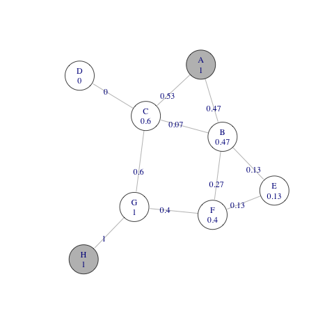
$$F_{i}^{(s,t)} = \frac{1}{2} \sum_j A_{i,j} |G_{i,s}^{+} - G_{i,t}^{+} + G_{j,t}^{+} - G_{j,s}^{+}|$$ The the current flow $F_{i}^{(s,t)}$ can be also expressed in terms of resistance distance as follows: $$ F_{i}^{(s,t)} = \frac{1}{4} \sum_j A_{i,j} |R_{i,s} - R_{i,t} + R_{j,t} - R_{j,s} |. $$The next figure gives an example. Each node is now labelled with the value of flow through it when a unit current is injected in node A and removed from node H. Each edge is labelled with the absolute current flowing on it. Notice that the flow from A to H through node G is 1 (all paths from A to H pass eventually through G), the flow through F is 0.4 (a proper subset of the paths from A to H go through F and these paths are generally longer than for G), and the flow through E is 0.13 (a proper subset of the paths from A to H go through E and these paths are generally longer than for F).
Finally, the current-flow betweenness centrality $b_i$ of node $i$ is the flow through $i$ averaged over all source-target pairs $(s,t)$:
$\displaystyle{b_i = \frac{\sum_{s < t} F_{i}^{(s,t)}}{(1/2) n (n-1)}}$
The computational complexity of computing current-flow centrality measures is the sum of the complexity of finding $G^+$, hence that of inverting a matrix of size the number of nodes of the graph, and the complexity of computing the centrality scores using the entries of $G^+$. Inverting a matrix of size $n$ costs $O(n^3)$. Computing the closeness scores costs $O(n)$, while computing the betweenness scores costs $O(n^2 (n+m))$. Hence, the complexity of current-flow closeness is $O(n^3)$ and that for current-flow betweenness is $O(n^2 (n+m))$ . This both for unweighted and weighted graphs. On the other hand, shortest-path measures cost $O(n (n+m))$ in the unweighted case, and $O(nm + n^2 \log n)$ in the weighted case.
# Invert reduced Laplacian matrix
# Input: an adjacency matrix A of an undirected graph
# Output: the inverted reduced Laplacian matrix
irl = function(A) {
  # number of nodes
  n = dim(A)[1]

  # ignore self-edges
  diag(A) = 0

  # get Laplacian matrix
  L = -A
  diag(L) = A %*% rep(1,n)

  # get reduced Laplacian matrix by removing first row and column
  L = L[-1,-1]

  # invert reduced Laplacian matrix
  L = solve(L)

  # add first row and column of all 0s
  L = rbind(0,L)
  L = cbind(0,L)

  return(L)
}

# Computes resistance distance matrix
# Input: an adjacency matrix A of an undirected graph
# Output: resistance distance matrix
resistance = function(A) {

  # number of nodes
  n = dim(A)[1]

  # invert reduced Laplacian
  L = irl(A)

  # compute resistance matrix
  e = rep(1, n)
  R = e %*% t(diag(L)) + diag(L) %*% t(e) - 2*L

  return(R)
}

# Computes current-flow closeness centrality
# Input: an adjacency matrix A of an undirected graph
# Output: a vector with the centrality score for each node
cfc = function(A) {

  # number of nodes
  n = dim(A)[1]

  # invert reduced Laplacian
  R = resistance(A)

  # compute centralities
  c = 1 / rowMeans(R)

  return(c)
}


# Computes current-flow betweenness centrality
# Input: an adjacency matrix A of an undirected graph
# Output: a vector with the centrality score for each node
cfb = function(A) {

  # number of nodes
  n = dim(A)[1]

  # invert reduced Laplacian
  R = resistance(A)

  # compute centralities
  f = 0
  b = rep(0,n)
  for (i in 1:n) {
    #compute neighborhood of i
    nei = which(A[i,] != 0)
    for (s in 1:(n-1)) {
      for (t in (s+1):n) {
        if ((s == i) | (t == i)) {
          f = 1
        }
        else {
          x = A[i,nei]
          y = abs((R[s,i] - R[t,i]) - (R[s,nei] - R[t,nei]))
          f = (x %*% y) / 4
        }
        b[i] = b[i] + f
      }
    }
    b[i] = 2 * b[i] / (n * (n-1))
  }

  return(b)
}