European natural gas pipeline network
We work on the European natural gas pipeline network. Data comes from the website of the International Energy Agency. The network is depicted here: European natural gas pipeline network. The nodes of the network are countries and the edges are directed pipes weighted with maximum flow.
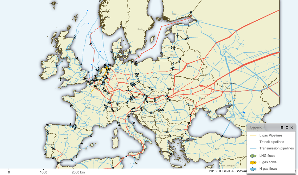
Data challenges
on the undirected unweighted network, compute and compare Katz centrality and power. In particular, identify powerful contries that are not central and central countries that are not powerful. Moreover, plot the network with node size proportional to power and centrality and visually compare the two graphs;
on the undirected weighted network, plot the network with edge with proportional to the edge weight (pipeline maxflow). Compute and compare power and centrality. Moreover, plot the network with node size proportional to power and centrality and visually compare the two graphs;
on the directed weighted network, plot the network with edge with proportional to the edge weight (pipeline maxflow). Compute centrality and strength (we do not have a notion of power in the directed case) on both the original graph (where edge direction indicates the flow of energy or importations) and the inverted one (where edge direction indicates the flow of money or exportations). Identify exporters that are not importers and importers that are not exporters.
Load libraries and user-defined functions:
library(igraph)
library(lpSolve)
library(lpSolveAPI)

# Compute power x = (1/x) A
#INPUT
# A = graph adjacency matrix
# t = precision
# OUTPUT
# A list with:
# vector = power vector
# iter = number of iterations

power = function(A, t) {
  n = dim(A)[1];
  # x_2k
  x0 = rep(0, n);
  # x_2k+1
  x1 = rep(1, n);
  # x_2k+2
  x2 = rep(1, n);
  diff = 1
  eps = 1/10^t;
  iter = 0;
  while (diff > eps) {
    x0 = x1;
    x1 = x2;
    x2 = (1/x2) %*% A;
    diff = sum(abs(x2 - x0));
    iter = iter + 1;
  }
  # it holds now: alpha x2 = (1/x2) A
  alpha = ((1/x2) %*% A[,1]) / x2[1];
  # hence sqrt(alpha) * x2 = (1/(sqrt(alpha) * x2)) A
  x2 = sqrt(alpha) %*% x2;
  return(list(vector = as.vector(x2), iter = iter))
}

# Verify if a graph is regularizable and, in case, gives the regularization solution using linear programming
#INPUT
# g = the graph
# OUTPUT
# A list with:
# w = weights for the edges
# d = regularization degree
regularify = function(g) {
  n = vcount(g)
  m = ecount(g)
  E = get.edges(g, E(g))
  B = matrix(0, nrow = n, ncol = m)
  # build incidence matrix
  for (i in 1:m) {
    B[E[i,1], i] = 1
    B[E[i,2], i] = 1
  }
  # objective function
  obj = rep(0, m + 1)
  # constraint matrix
  con = cbind(B, rep(-1, n))
  # direction of constraints
  dir = rep("=", n)
  # right hand side terms
  rhs = -degree(g)
  # solve the LP problem
  sol = lp("max", obj, con, dir, rhs)
  # get solution
  if (sol$status == 0) {
    s = sol$solution
    # weights
    w = s[1:m] + 1
    # weighted degree
    d = s[m+1]
  }
  # return the solution
  if (sol$status == 0) return(list(weights = w, degree = d)) else return(NULL)
}
Read the dataset
# read states and abbreviations
dfstates = read.table("states.csv", header = TRUE, sep = "", stringsAsFactors = FALSE)
states = dfstates[,"State"]
abb.states = dfstates[,"Abbreviation"]

# read edges and weights
df = read.table("IEA.csv", header = TRUE, sep = ";", stringsAsFactors = FALSE)
entry = df[,"Entry"]
exit = df[,"Exit"]
Create graphs
The original data corresponds to a directed, weighted multigraph, with edge weights corresponding to the maximum flow of the pipeline. We will create four networks from the original data.
# create directed weighted graph (dwg)
el = cbind(exit, entry)
dwg = graph_from_edgelist(el, directed = TRUE)
E(dwg)$weight = df[,"Maxflow"]

# remove Liquefied Natural Gas (LNG) node
dwg = delete_vertices(dwg, 1)

# simplify network (we sum edge weights of multiple edges)
dwg = simplify(dwg, edge.attr.comb="sum")

# create directed unweighted graph (dug)
dug = dwg
dug = delete_edge_attr(dug, "weight")

# create undirected weighted graph (uwg)
# If edges are reciprocal, edge weightes are summed
uwg = as.undirected(dwg, mode = "collapse", edge.attr.comb="sum")

# create undirected unweighted graph (uug)
uug = uwg
uug = delete_edge_attr(uug, "weight")
Analyze undirected unweighted network
Let’s start by analysing the most simple model: the undirected unweighted graph.
Plot network
# plot network with country abbreviations
plot(uug, vertex.size=10, vertex.shape = "none", vertex.label=abb.states)
Compute power and centrality
We will use Katz measure as a representant for centrality and power measure as a representant for power.
# Centrality (Katz)
A = as_adjacency_matrix(uug)
eig = eigen(A)$values
r = max(abs(eig))
alpha = 0.85 / r
c =  alpha_centrality(uug, alpha = alpha)
names(c) = states

# Power
# The graph is not regularizable
regularify(uug)
## NULL# Use diagonal perturbation
A = as_adjacency_matrix(uug)
damping = 0.15
n = vcount(uug)
I = diag(damping, n)
Ad = A + I
p = power(Ad, 6)$vector
names(p) = statesCompare power and centrality
summary(c)## Min. 1st Qu. Median Mean 3rd Qu. Max.
## 1.406 1.855 3.003 3.935 5.052 12.755hist(c, main = "", xlab = "Centrality")
summary(p)## Min. 1st Qu. Median Mean 3rd Qu. Max.
## 0.4754 0.6063 1.5226 2.0615 2.9509 6.2565hist(p, main = "", xlab = "Power")
# sort top-10 states according to centrality
round(sort(c, decreasing=TRUE)[1:10], 3)
## Germany Norway Belgium Austria Netherlands
## 12.755 8.666 8.445 7.997 7.648
## France Switzerland Denmark Czech Republic United Kingdom
## 7.324 6.349 6.012 5.912 5.297# sort top-10 states according to power
round(sort(p, decreasing=TRUE)[1:10], 2)## Turkey Germany Italy Spain Hungary
## 6.26 6.09 5.54 5.50 4.62
## Russia Bulgaria Belgium Austria United Kingdom
## 4.53 3.99 3.60 3.29 3.09# sort bottom-10 states according to centrality
round(sort(c, decreasing=FALSE)[1:10], 3)## Macedonia Portugal Morocco Iran Georgia Moldova Serbia
## 1.406 1.477 1.477 1.485 1.485 1.496 1.803
## Finland Libya Algeria
## 1.813 1.816 1.817# sort bottom-10 states according to power
round(sort(p, decreasing=FALSE)[1:10], 2)## Iran Georgia Libya Portugal Morocco Serbia Finland
## 0.48 0.48 0.49 0.49 0.49 0.51 0.51
## Macedonia Ireland Sweden
## 0.53 0.58 0.59# correlation
cor(c, p, method="kendall")## [1] 0.5745721# scatterplot
mc = quantile(c, 0.75)
mp = quantile(p, 0.75)
color = rgb(0, 0, 0, 0.5)
plot(p, c, xlab="power", ylab="centrality", pch=NA, bty="l")
text(p, c, labels=abb.states, adj=c(0.5,0.5), cex=1, col = color)
abline(h=mc, lty=2)
abline(v=mp, lty=2)
# plot networks with node size proportional to power
coords = layout_with_fr(uug)
sp = 12 * p / max(p)
plot(uug, layout=coords, vertex.color="red", vertex.label= NA, vertex.size = sp, edge.width=2, edge.color="black")
# plot networks with node size proportional to centrality
sc = 12 * c / max(c)
plot(uug, layout=coords, vertex.color="red", vertex.label= NA, vertex.size = sc, edge.width=2, edge.color="black")
Analyze undirected weighted network
Plot network
We plot the network with edge width proportional to weight (pipeline maxflow). We replaced unknown weights (NA) with the mean weight.
w = E(uwg)$weight
m = mean(w, na.rm=TRUE)
w[is.na(w)] = m
plot(uwg, layout = layout_with_gem(uwg), vertex.size=10, vertex.shape = "none", vertex.label=abb.states, edge.width = 0.5*w)
Compute power and centrality
Some pipeline maxflows (edge weights) are unknown. We decided to assign the mean maxflow to edges with unknown maxflow.
# Centrality (Katz)
# assign mean maxflow to edges with unknown maxflow
w = E(uwg)$weight
m = mean(w, na.rm=TRUE)
w[is.na(w)] = m
E(uwg)$weight = w
A = as_adjacency_matrix(uwg, sparse=TRUE, attr="weight")
eig = eigen(A)$values
r = max(abs(eig))
alpha = 0.85 / r
c =  alpha_centrality(uwg, alpha = alpha)
names(c) = states

# Power
A = as_adjacency_matrix(uwg, sparse=TRUE, attr="weight")
damping = 0.15
n = vcount(uwg)
I = diag(damping, n)
Ad = A + I
p = power(Ad, 6)$vector
names(p) = states
Compare power and centrality
# sort top-10 states according to centrality
round(sort(c, decreasing=TRUE)[1:10], 3)
## Germany Czech Republic Slovak Republic Poland
## 11.250 10.740 6.488 4.001
## Ukraine Russia Norway Austria
## 3.959 3.930 3.929 3.552
## Belgium Netherlands
## 3.304 2.984# sort top-10 states according to power
round(sort(p, decreasing=TRUE)[1:10], 2)## Germany Turkey Italy Romania
## 14.94 12.19 10.11 7.90
## Slovak Republic Spain Latvia United Kingdom
## 7.78 6.28 6.21 5.16
## Hungary Norway
## 4.10 4.05# sort bottom-10 states according to centrality
round(sort(c, decreasing=FALSE)[1:10], 3)## Macedonia Sweden Greece Portugal Serbia Slovenia
## 1.005 1.021 1.031 1.045 1.046 1.072
## Morocco Croatia Ireland Luxembourg
## 1.075 1.085 1.100 1.104# sort bottom-10 states according to power
round(sort(p, decreasing=FALSE)[1:10], 2)## Macedonia Luxembourg Serbia Libya Portugal Sweden
## 0.42 0.43 0.46 0.47 0.47 0.47
## Iran Georgia Ireland Finland
## 0.50 0.50 0.53 0.53# correlation
cor(c, p, method="kendall")## [1] 0.5702076# scatterplot
mc = quantile(c, 0.75)
mp = quantile(p, 0.75)
color = rgb(0, 0, 0, .5)
plot(p, c, xlab="power", ylab="centrality", pch=NA, bty="l")
text(p, c, labels=abb.states, adj=c(0.5,0.5), cex=1, col = color)
abline(h=mc, lty=2)
abline(v=mp, lty=2)
# plot networks with node size proportional to power
# save coordinates
coords = layout_with_fr(uwg)
sp = 12 * p / max(p)
plot(uwg, layout=coords, vertex.color="red", vertex.label= NA, vertex.size = sp, edge.width=2, edge.color="black")
# plot networks with node size proportional to centrality
sc = 12 * c / max(c)
plot(uwg, layout=coords, vertex.color="red", vertex.label= NA, vertex.size = sc, edge.width=2, edge.color="black")
Analyze directed weighted network
Plot network
We plot the network with edge width proportional to weight (pipeline maxflow). We replaced unknown weights (NA) with the mean weight.
w = E(dwg)$weight
m = mean(w, na.rm=TRUE)
w[is.na(w)] = m
plot(dwg, layout = layout_with_gem(dwg), vertex.size=4, vertex.shape = "none", edge.arrow.size=0.2, vertex.label=abb.states, edge.width = 0.5 * w)
Compute centrality
We have two options: a country is central if it imports from central ones or a country is central if it exports from central ones. Notice that the direction of the flow of money is opposite with respect to the direction of the flow of gas (hence the second definition makes more sense).
# Centrality (Katz)
w = E(dwg)$weight
m = mean(w, na.rm=TRUE)
w[is.na(w)] = m
E(dwg)$weight = w

# A country is central if it imports from central ones (uses in-edges)
A = as_adjacency_matrix(dwg, sparse=FALSE, attr="weight")
eig = eigen(A)$values
r = max(abs(eig))
alpha = 0.85 / r
c1 =  alpha_centrality(dwg, alpha = alpha)
names(c1) = states

# Or: a country is central if it exports to central ones (uses out-edges)
# rotate the matrix in the direction of flow of money
A2 = t(A)
g = graph_from_adjacency_matrix(A2, weighted=TRUE)
eig = eigen(A2)$values
r = max(abs(eig))
alpha = 0.85 / r
c2 =  alpha_centrality(g, alpha = alpha)
names(c2) = states

# sort central importers and exporters
round(sort(c1, dec=TRUE)[1:10], 3)
## Czech Republic Germany Slovak Republic Austria
## 15.372 14.046 6.581 6.265
## Belgium Netherlands Switzerland Italy
## 5.407 4.838 4.725 4.673
## France Poland
## 4.342 4.093round(sort(c2, dec=TRUE)[1:10], 3)## Germany Czech Republic Slovak Republic Norway
## 10.492 9.431 8.357 8.208
## Ukraine Russia Poland Netherlands
## 7.671 6.387 5.257 4.850
## Belgium Austria
## 4.289 4.055# correlation
cor(c1, c2, method="kendall")## [1] 0.4597451# scatterplot
mc1 = quantile(c1, 0.75)
mc2 = quantile(c2, 0.75)
color = rgb(0, 0, 0, .5)
plot(c1, c2, xlab="import", ylab="export", pch=NA, bty="l")
text(c1, c2, labels=abb.states, adj=c(0.5,0.5), cex=1, col = color)
abline(h=mc1, lty=2)
abline(v=mc2, lty=2)
Compute strength
# importers
s1 = strength(dwg, mode="in")
# exporters
s2 = strength(dwg, mode="out")

# sort central importers and exporters
round(sort(s1, dec=TRUE)[1:10], 3)
## Germany Czech Republic Slovak Republic Italy
## 28.185 18.968 15.825 14.120
## United Kingdom Belgium Austria Netherlands
## 11.520 10.913 10.328 9.788
## France Poland
## 8.695 7.728round(sort(s2, dec=TRUE)[1:10], 3)## Germany Norway Ukraine Slovak Republic
## 20.205 19.635 16.270 15.838
## Czech Republic Russia Austria Belgium
## 12.968 10.518 9.688 9.193
## Netherlands United Kingdom
## 8.103 7.455# correlation
cor(c1, c2, method="kendall")## [1] 0.4597451# scatterplot
ms1 = quantile(s1, 0.75)
ms2 = quantile(s2, 0.75)
color = rgb(0, 0, 0, .5)
plot(s1, s2, xlab="import", ylab="export", pch=NA, bty="l")
text(s1, s2, labels=abb.states, adj=c(0.5,0.5), cex=1, col = color)
abline(h=ms1, lty=2)
abline(v=ms2, lty=2)