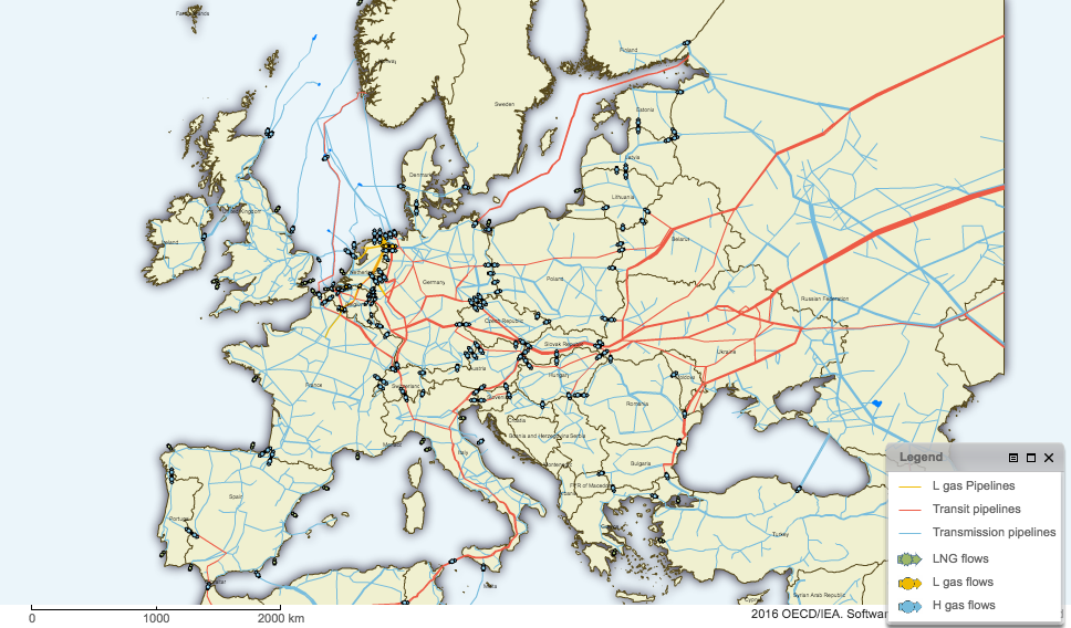
European natural gas pipeline network

We work on the European natural gas pipeline network. Data comes from the website of the International Energy Agency. The network is depicted here: European natural gas pipeline network. The nodes of the gas network are countries and the edges are undirected pipes weighted with cumulative gas flow.

Dataset

XML encoding of the gas network: gas.xml

Data challenges

On the gas network, compute and compare Katz centrality and power. In particular, identify powerful contries that are not central and central countries that are not powerful. Moreover, plot the network with node size proportional to power and centrality and edge width proportional to gas flow.

Load libraries and user-defined functions:

library(dplyr)
library(ggplot2)
library(igraph)
library(tidygraph)
library(ggraph)
library(lpSolve)
library(lpSolveAPI)

# Compute power x = (1/x) A 
#INPUT
# A = graph adjacency matrix
# t = precision
# OUTPUT
# A list with:
# vector = power vector
# iter = number of iterations

power = function(A, t) {
  n = dim(A)[1];
  # x_2k
  x0 = rep(0, n);
  # x_2k+1
  x1 = rep(1, n);
  # x_2k+2
  x2 = rep(1, n);
  diff = 1
  eps = 1/10^t;
  iter = 0;
  while (diff > eps) {
    x0 = x1;
    x1 = x2;
    x2 = (1/x2) %*% A;
    diff = sum(abs(x2 - x0));
    iter = iter + 1;
  } 
  # it holds now: alpha x2 = (1/x2) A
  alpha = ((1/x2) %*% A[,1]) / x2[1];
  # hence sqrt(alpha) * x2 = (1/(sqrt(alpha) * x2)) A
  x2 = sqrt(alpha) %*% x2;
  return(list(vector = as.vector(x2), iter = iter))
}  

# read the gas network
gas = read_graph(file="gas.xml", format="graphml")
gas = delete_vertex_attr(gas, "id")

Compute power and centrality

# Centrality (Katz)
A = as_adjacency_matrix(gas, sparse=TRUE, attr="weight")
eig = eigen(A)$values
r = max(abs(eig))
alpha = 0.85 / r
c =  alpha_centrality(gas, alpha = alpha)
V(gas)$centrality = c

# Power
A = as_adjacency_matrix(gas, sparse=TRUE, attr="weight")
damping = 0.15
n = vcount(gas)
I = diag(damping, n)
Ad = A + I
p = power(Ad, 6)$vector
names(p) = names(c)
V(gas)$power = p

Compare power and centrality

# sort top-5 states according to centrality
round(sort(c, decreasing=TRUE)[1:5], 3)

##        Germany    Netherlands Czech Republic        Belgium         Norway 
##         11.628          8.410          7.975          6.050          4.961

# sort top-5 states according to power
round(sort(p, decreasing=TRUE)[1:5], 2)

##         Germany           Italy Slovak Republic          Turkey           Spain 
##           18.56           10.86           10.06            6.84            6.16

# correlation
cor(c, p, method="kendall")

## [1] 0.6214896

nodes = as_data_frame(gas, what="vertices")

# 3rd quantiles
q_centrality = quantile(nodes$centrality, 0.75)
q_power = quantile(nodes$power, 0.75)

ggplot(nodes, aes(x = centrality, y = power)) +
  geom_text(aes(label = short_name), alpha = 0.5) +
  geom_hline(yintercept = q_power, alpha = 0.5, lty = 2) +
  geom_vline(xintercept = q_centrality, alpha = 0.5, lty = 2)

# neighbors of Italy
edges = as_data_frame(gas, what="edges")

edges %>% 
  filter(from == "Italy") %>% 
  left_join(nodes, join_by(to == name))

##    from          to   weight short_name centrality     power
## 1 Italy     Austria 5.370000         AT   3.252255 2.7825805
## 2 Italy Switzerland 3.708815         CH   2.173446 1.3798099
## 3 Italy     Croatia 0.670000         HR   1.053107 0.6700288
## 4 Italy     Tunisia 4.400000         TN   1.349537 2.9767098
## 5 Italy       Libya 1.460000         LY   1.074091 0.4603354
## 6 Italy    Slovenia 0.380000         SI   1.049107 0.6610395

edges %>% 
  filter(to == "Italy") %>% 
  left_join(nodes, join_by(from == name))

## [1] from       to         weight     short_name centrality power     
## <0 rows> (or 0-length row.names)

gas_tbl = as_tbl_graph(gas, directed = FALSE)

seed = 99
set.seed(seed)
ggraph(gas_tbl, layout = "lgl") + 
  geom_edge_link(aes(alpha = weight)) + 
  geom_node_point(aes(size = centrality)) +
  geom_node_text(aes(label = short_name), repel=TRUE) +
  theme_graph()

set.seed(seed)
ggraph(gas_tbl, layout = "lgl") + 
  geom_edge_link(aes(alpha = weight)) + 
  geom_node_point(aes(size = power)) +
  geom_node_text(aes(label = short_name), repel=TRUE) +
  theme_graph()