The simplest and oldest network model is the random model, also known as Erdős-Rényi model. According to this model, a network is generated by laying down a number $n$ of nodes and adding edges between them with independent probability $p$ for each node pair.
n = 100
p = 1.5/n
g.erdos.renyi = erdos.renyi.game(n, p)

coords = layout.fruchterman.reingold(g.erdos.renyi)
coords3D = layout.fruchterman.reingold(g.erdos.renyi, dim=3)

plot(g.erdos.renyi, layout=coords, vertex.size = 3, vertex.label=NA)
tkplot(g.erdos.renyi, layout=coords, vertex.label = NA, vertex.size=3)
rglplot(g.erdos.renyi, layout=coords3D, vertex.label = NA, vertex.size=3)
This model generates a small world network: the average geodesic distance is $d = \log n / \log p(n-1)$. For instance, if we have 1000 nodes and we add links with probability $0.01$, network nodes have on average only 3 degrees of separation. To grasp the logarithmic mean geodesic distance consider a typical node in the random network. This node has $k = p (n-1)$ edges and hence can directly reach $k$ nodes. There are, moreover, about $k^2$ nodes two links away and roughly $k^d$ nodes exactly $d$ links away. Hence, in order to reach all $n$ nodes in the network, we need $d = \log n / \log k$ steps, which is a very small number compared to $n$.
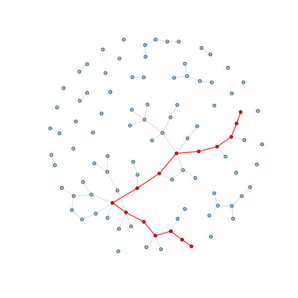
Let's check the average geodesic distance and the diameter (the largest geodesic distance) of the generated random graph:
average.path.length(g.erdos.renyi)
[1] 5.773585

d = get.diameter(g.erdos.renyi)
length(d) - 1
[1] 14

E(g.erdos.renyi)$color = "grey"
E(g.erdos.renyi)$width = 1
E(g.erdos.renyi, path=d)$color = "red"
E(g.erdos.renyi, path=d)$width = 2
V(g.erdos.renyi)$color  = "SkyBlue2"
V(g.erdos.renyi)[d]$color = "red"
plot(g.erdos.renyi, layout=coords, vertex.label = NA, vertex.size=3)
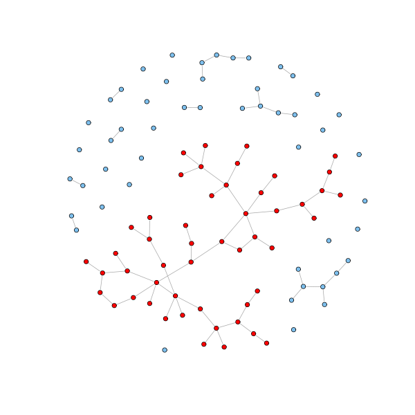
Furthermore, if $p \geq 1/n$, then a giant component emerges capturing the majority of the nodes.
# Get the clusters
cl = clusters(g.erdos.renyi)

# How many components?
cl$no
[1] 31

# How big are these?
table(cl$csize)

 1  2  5  7 50
21  6  2  1  1

# Get the giant component
nodes = which(cl$membership == which.max(cl$csize) - 1) - 1

V(g.erdos.renyi)$color  = "SkyBlue2"
V(g.erdos.renyi)[nodes]$color = "red"
plot(g.erdos.renyi, layout=coords, vertex.size = 3, vertex.label=NA)
Unfortunately, the analogies with most real networks abruptly stop here. The clustering coefficient, the probability that the neighbour of my neighbour is also my neighbour, is $p$, that is the probability that any two random nodes are connected. This is unrealistic.
g = erdos.renyi.game(1000, 4/1000)

transitivity(g)
[1] 0.004001455
Furthermore, the probability $P(k)$ that a node has $k$ neighbours is the binomial:
$\displaystyle{P(k) = {{n-1} \choose k} p^k (1-p)^{n-1-k}}$
which can be approximated by the Poisson distribution:
$\displaystyle{P(k) = \frac{\lambda^k e^{-\lambda}}{k!}}$
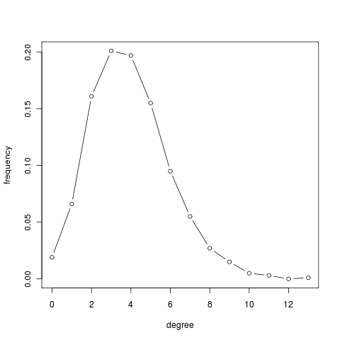
for large values of $n$ and small values of $p$, where $\lambda = p(n-1)$. The Poisson distribution is peaked at the average degree $\lambda$: the majority of nodes have the same typical degree and nodes deviating from the average are extremely rare. In other words, a random network has a characteristic scale, which contrasts with the scale-free nature of real webs.
g = erdos.renyi.game(1000, 4/1000)

deg = degree(g)
summary(deg)
   Min. 1st Qu.  Median    Mean 3rd Qu.    Max.
  0.000   3.000   4.000   3.956   5.000  13.000

deg.dist = degree.distribution(g)
deg.dist
 [1] 0.01900000 0.06600000 0.16100000 0.20100000 0.19700000 0.15500000
 [7] 0.09500000 0.05500000 0.02700000 0.01500000 0.00500000 0.00300000
[13] 0.00000000 0.00100000

plot(0:max(deg), deg.dist , xlab="degree", ylab="frequency", type="b")
The model proposed by Watts and Strogatz was the first attempt to reconcile small world and high clustering under the same umbrella. They started with a circle of nodes, where each node is connected to its nearest neighbours as well as to its next-nearest neighbours.
g = watts.strogatz.game(1, 10, 2, 0)

plot(g, layout=layout.circle, vertex.label=NA)
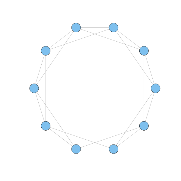
Each node in the model has 4 neighbours, and these are connected to each other with 3 links. If all 4 neighbours were connected to each other, there would be 6 links. Hence, the clustering coefficient is 0.5, which is much higher than the coefficient for a random network in which the typical node has 4 links. Indeed, if such a random network has $n$ nodes, then the clustering coefficient is $p = \langle k \rangle / (n-1)$, where $\langle k \rangle$ is the average number of links of a node, and $n-1$ represents the maximum number of links of a node. Clearly, if $\langle k \rangle$ is fixed, the clustering coefficient $p$ vanishes as $n$ grows. Hence, Watts-Strogatz model is highly clustered.
However, it is not a small world. To get to a node, one has to travel across many nodes on average. To make this world a small one, the authors rewired a few extra links connecting randomly selected nodes.
g = watts.strogatz.game(1, 10, 2, 0.2)

plot(g, layout=layout.circle, vertex.label=NA)
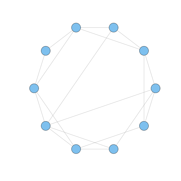
The surprising finding is that even a few extra links are sufficient to drastically decrease the geodesics between nodes, without significantly changing the clustering property.
g = watts.strogatz.game(1, 1000, 2, 0)

average.path.length(g)
[1] 125.3754

transitivity(g)
[1] 0.5

g = watts.strogatz.game(1, 1000, 2, 0.1)

average.path.length(g)
[1] 6.958456

transitivity(g)
[1] 0.2495667

transitivity(erdos.renyi.game(vcount(g), ecount(g), type = "gnm"))
[1] 0.003718394
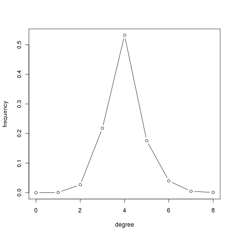
Watts-Strogatz model is interesting because offered a compromise between the random world of Erdős and Rényi, which is small but not transitive, and a regular lattice, which is clustered but has distant nodes. Moreover, it formalizes Granovetter's vision of the society. Unfortunately, this model fails to capture an essential feature of real networks: the power law distribution of node degrees. Indeed, all nodes have approximately the same number of edges.
deg.dist = degree.distribution(g)
deg.dist
[1] 0.000 0.001 0.027 0.218 0.532 0.176 0.040 0.005 0.001

plot(0:max(deg), deg.dist , xlab="degree", ylab="frequency", type="b")
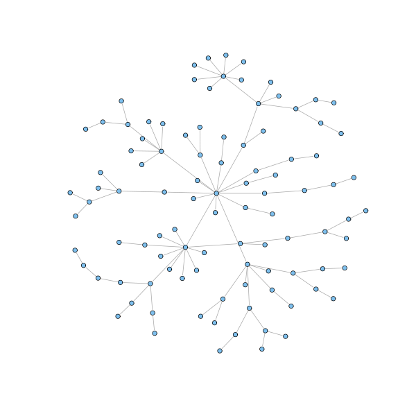
A network model that captures the power law distribution of node degrees is de Solla Price cumulative advantage, which was later rediscovered and further investigated under the name preferential attachment by Barabási and Albert. Such a model has the following two main ingredients:
Clearly, senior nodes have more chances to be connected than latecomers. However, seniority is not sufficient to explain the power law distribution, in particular the presence of hubs. These require the help of the second ingredient, the preferential attachment. As we all experienced in our lives, success breeds success, and popularity is attractive. Hence, nodes with a rich number of links will get even richer, while poor nodes are poised to remain in the dark land of obscurity. This closely resembles the following line in Jesus' parable of the talents in the biblical Gospel according to Matthew: For unto every one that hath shall be given, and he shall have abundance: but from him that hath not shall be taken away even that which he hath.
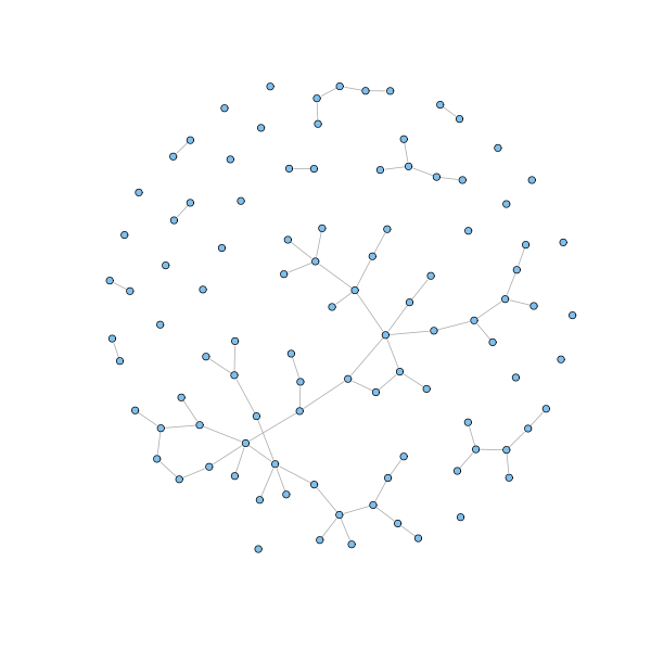
g = barabasi.game(100, m = 1, directed=FALSE, out.pref = TRUE)

plot(g, layout=layout.fruchterman.reingold, vertex.size=3, vertex.label=NA)
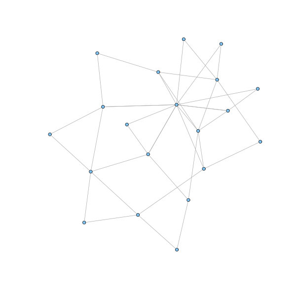
g = barabasi.game(20, m = 2, directed=FALSE, out.pref = TRUE)

plot(g, layout=layout.fruchterman.reingold, vertex.size=3, vertex.label=NA)
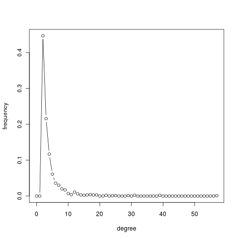
The described model generates a network whose node degrees asymptotically follow a power law distribution with exponent parameter equal to 3. Moreover, the presence of hubs keeps the network small: to get of a node, the shortest way is usually to pass through a highly connected hub. To be sure, we all experienced this when flying to a remote destination. Finally, the clustering coefficient can be proved to be higher than for random graphs, although it vanishes as the size of the networks grows.
g = barabasi.game(1000, m = 2, directed=FALSE, out.pref = TRUE)

average.path.length(g)
[1] 4.339706

transitivity(g)
[1] 0.007000206

transitivity(erdos.renyi.game(vcount(g), ecount(g), type = "gnm"))
[1] 0.002690238

deg = degree(g)
summary(deg)
   Min. 1st Qu.  Median    Mean 3rd Qu.    Max.
  2.000   2.000   3.000   3.996   4.000  57.000

deg.dist = degree.distribution(g)
deg.dist
 [1] 0.000 0.000 0.447 0.216 0.117 0.061 0.036 0.030 0.020 0.017 0.007 0.004
[13] 0.011 0.006 0.003 0.002 0.003 0.004 0.003 0.003 0.000 0.000 0.002 0.000
[25] 0.001 0.001 0.000 0.000 0.000 0.001 0.000 0.002 0.000 0.000 0.000 0.000
[37] 0.000 0.000 0.000 0.002 0.000 0.000 0.000 0.000 0.000 0.000 0.000 0.000
[49] 0.000 0.000 0.000 0.000 0.000 0.000 0.000 0.000 0.000 0.001

plot(0:max(deg), deg.dist , xlab="degree", ylab="frequency", type="b")