[home]
Mathematica notebooks available for download:
To see the files you will need MathematicaPlayer, a free utility from Wolfram Research. To use them you must have access to Mathematica. You can download a Trial version of Mathematica for free and use it for 15 days.
Mathematica tutorials in Italian for Mathematica:
Old Mathematica tutorials in Italian for Mathematica version 5.2 or earlier:
Versions History:
2008-11-06: First release.
2009-01-15: With Mathematica version 7 the package now uses the Cone primitive to draw 3D arrows, and it can map StreamPlots onto a surface.
2009-02-01: With Mathematica version 7 you can now use the Oriented option with ListCurvePathPlot and ListLinePlot too.
2010-01-16: With Mathematica version 7 or later you can now use the Oriented option with BSplineCurve too.
2010-05-06: removed obsolete references to pre-Mathematica 6 CurvesGraphics code, and added a new example.
2010-10-13: added support for Tube objects as an alternative to Line in 3D.
2010-11-28: improved spline support.
2011-02-18: added support for ColorFunction in Oriented.
2011-12-20: fixed a bug in PlotCurveOnSurface3D.
2012-01-17: fixed some bugs involving Oriented, ColorFunction, ReverseOrientation, ArrowShaftLength, Arrowheads.
2012-03-23: restored the functionality of TextToGraphics, TextToGraphics3D and text on a surface to Mathematica version 8.
2013-04-15: added the new options HeadProportion3D and HeadScalingTransform3D, and deleted obsolete references to HeadWidth3D. Added new mechanisms so that the shape of 3D arrow cones should not be affected by the value of BoxRatios. Turned off the warning messages about unknown options in Plot etc. LinearPhasePlot2D is back in working order. Other minor fixes and improvements.
2013-04-17: added compatibility with PlotLegends of version 9.
2013-05-09: added SyntaxInformation declarations.
2014-10-04: fixed and improved TextToGraphics and TextToGraphics3D.
2015-02-01: I take advantage of the new computational geometry features of Mathematica version 10 to give a (finally!) satisfactory support for drawing polygon and text on a curved surface. Not just outlined, but filled text. The functions are the same for the user, but the underlying code is new, and the performance is much better. The documentation is updated.
2015-02-12: added code to take care of the case when two font characters overlap (which is not so unusual), a situation that wreaked havoc in the previous version when drawing them onto a curved surface; the workaround may not work with complicated overlaps, but these should be rare. Some parallelization helps speed up the drawing of text on a surface.
2015-02-16: added support for the "{x,y}\[Element]region" syntax of Mathematica 10.
2015-09-08: corrected the usage notes on TextToGraphics.
2015-11-14: the functions FilledCurveToLines and FilledCurveToPolygons, formerly private, are now available for outside use. Also, TextToGraphics, TextToGraphics3D and other text-drawing functions can now call an external routine for PDF conversion, using the PDFConversionFunction option.
2015-12-24: added a workaround for a bug in Mathematica 10.3.1.
2016-08-29: added OrientedPolarPlot and the Oriented option for PolarPlot.
2017-03-29: added the new option CurveParameterRange to improve appearance of curves that have arrows at the end. Corrected a bug in line clipping that could cause endless execution loops in such functions as PhasePlot.
2017-04-18: corrected a bug.
2017-05-09: corrected a bug.
2018-05-05: improved the documentation on TextToGraphics3D.
2020-01-15: added an option to give a thickness to TextToGraphics3D.
2021-04-21: updated TextToGraphics to deal with a change in behaviour of ImportString in Mathematica version 12.2.
2022-04-28: found a workaround for a WL bug affecting ContourLabels.
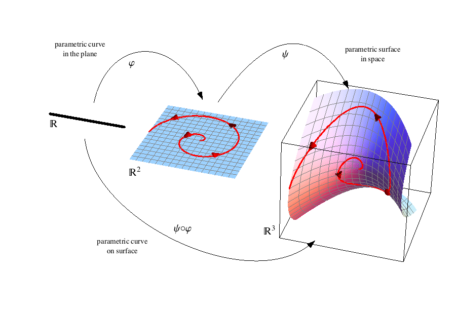
The package defined in the CurvesGraphics6 notebook adds the following capabilities to Mathematica graphics:
Number, positions, size, shape, style, color of the arrows and of the curves are customizable through options. The default values of the options have been chosen to give pleasing results in most typical cases that I could think of, with hardly any tweaking.
Obsolete versions: the precursors of CurvesGraphics6 are still available for download: ODEPlot, LevelPlot3D, CurveOnSurface. They don't need DrawGraphics. They have no 3D-arrow capability, and the interface is different. I tried to make DrawGraphics backward compatible with the older syntax, but I make no guarantee.
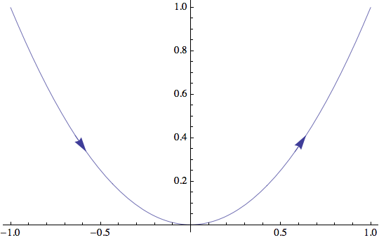
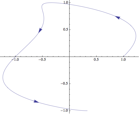
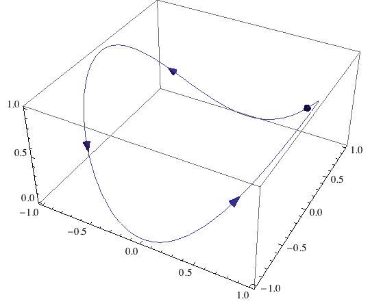
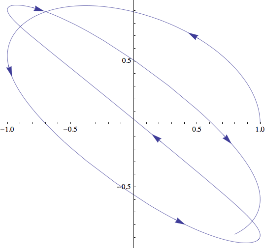
Basic examples of the option Oriented in the plane and in space:
Plot[x^2, {x, -1, 1}, Oriented->True]
ParametricPlot[{Cos[x] + Sin[3x]/3, Sin[x]}, {x, 0, 3Pi/2}, Oriented->True]
ParametricPlot3D[{Cos[t], Sin[t], Cos[t]^2}, {t, 0, 2Pi}, Oriented->True]
Basic examples of the option PlotSolution:
NDSolve[{x''[t] == -x[t](1 + x[t]^2), y''[t] == -y[t](1 + x[t]^2 - x[t]^4), x[0] == 1, y[0] == 0, x'[0] == 0, y'[0] == 1}, {x, y}, {t, 0, 10}, Plot->True]
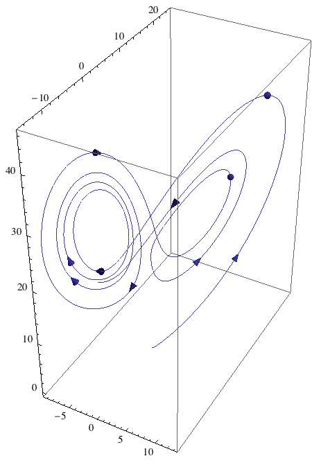
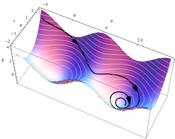
Plot of Lorenz's equations:
NDSolve[{x'[t] == -3 (x[t] - y[t]), y'[t] == -x[t] z[t] + 26.5 x[t] - y[t], z'[t] == x[t] y[t] - z[t], x[0] == z[0] == 0, y[0] == 1}, {x, y, z}, {t, 0, 9.1}, PlotSolution->True, HeadLength3D -> 1/30]
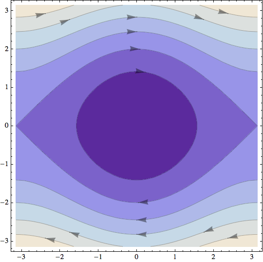
Basic oriented contour plot:
ContourPlot[-Cos[x] + y^2/2, {x, -Pi, Pi}, {y, -Pi, Pi}, Oriented->True]
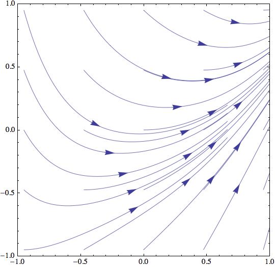
Basic phase plot:
PhasePlot[{1/(1 + x^2), -y + x}, {x, -1, 1}, {y, -1, 1}, {0, 2}]
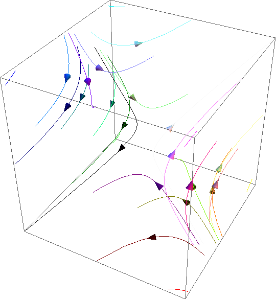
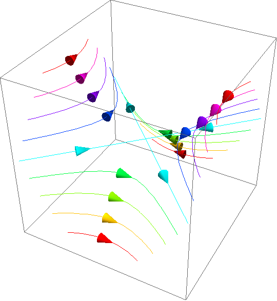
Basic phase plot in 3D space:
PhasePlot[{x + 2 y + 3 z, 4 x + 3 y + 2 z, 3 x + y + 2 z},{x, -1, 1}, {y, -1, 1}, {z, -1, 1},{-2,2},GridPoints -> 3, PlotStyle -> RGBColor]
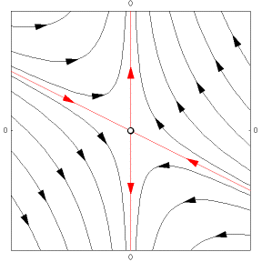
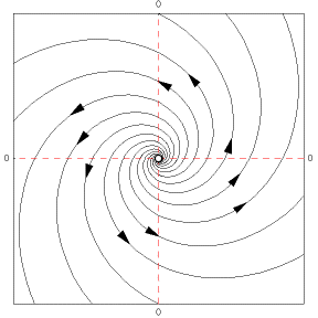
Phase plot for linear systems:
LinearPhasePlot[{{-1, 0}, {1, 1}}]
LinearPhasePlot[{{1/2, -1}, {1, 1/2}}]
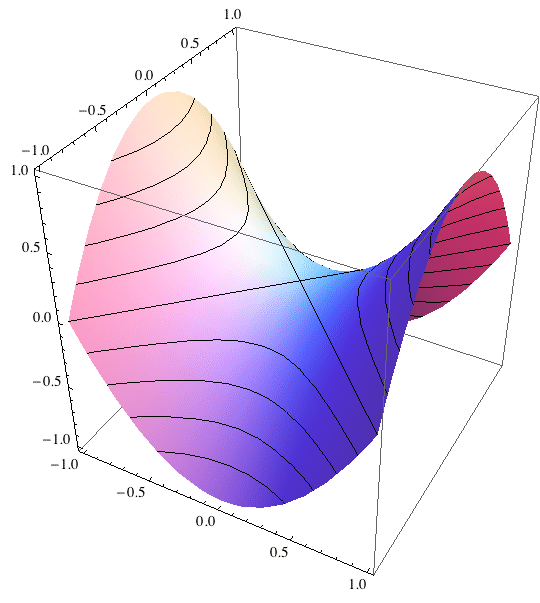
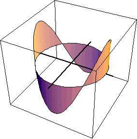
LevelPlot3D plots the level sets of a function in three dimensions:
LevelPlot3D[x^2 - y^2, {x, -1, 1}, {y, -1, 1}, BoxRatios -> {1, 1, 1}]
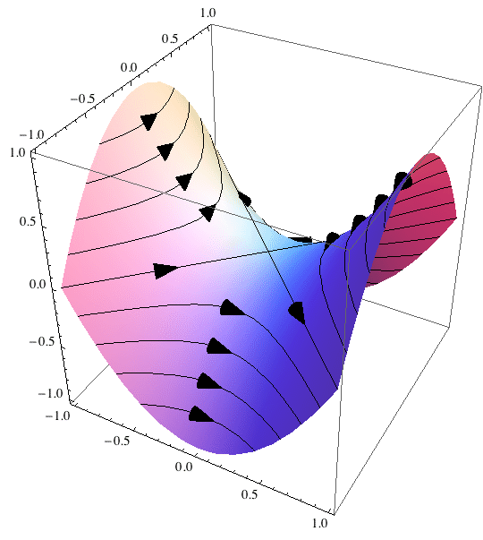
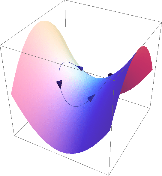
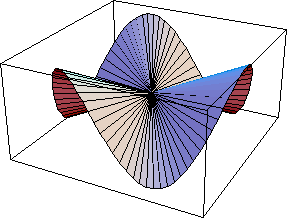
Oriented level lines:
LevelPlot3D[x^2 - y^2, {x, -1, 1}, {y, -1, 1}, Oriented -> True]
You can optionally get the level sets projected on a plane:
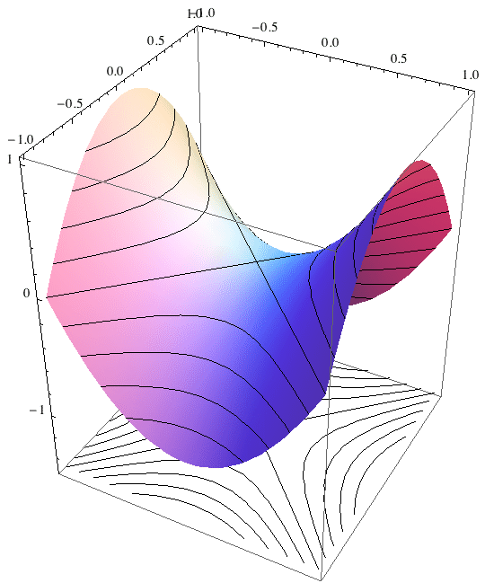
There are options for coloring the level lines according to elevation, and for suppressing the surface:
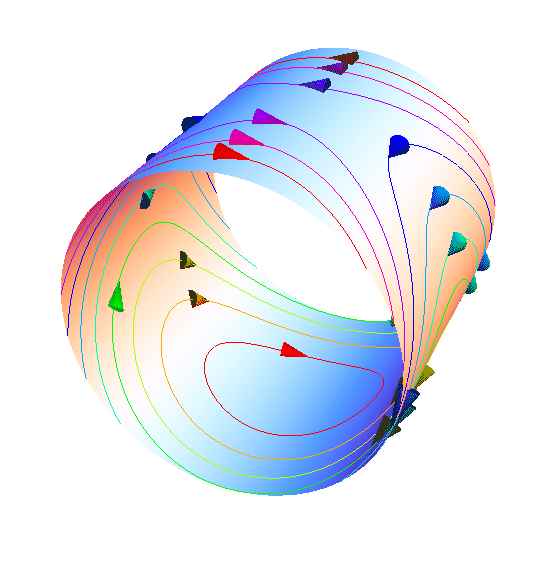
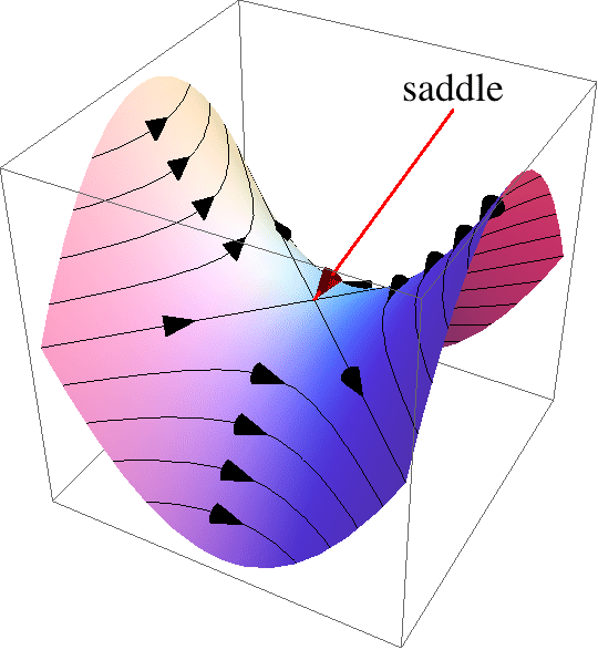
PlotCurveOnSurface3D basic examples:
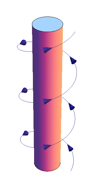
With CurvesGraphics6 it is easy to draw curves on a surface. Take for example an oriented curcle on a saddle:
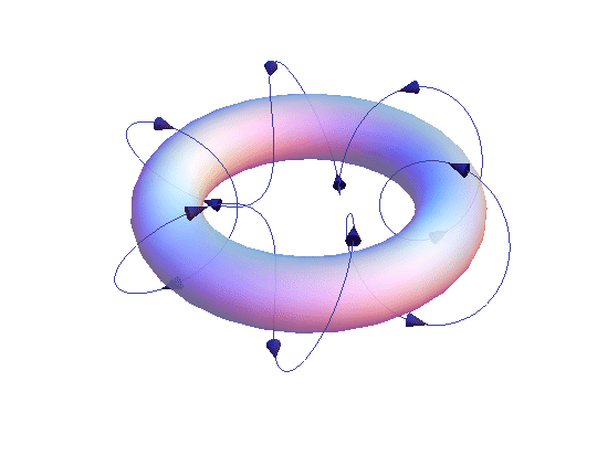
You can also draw more than one curve, and of different colors, on the same surface:
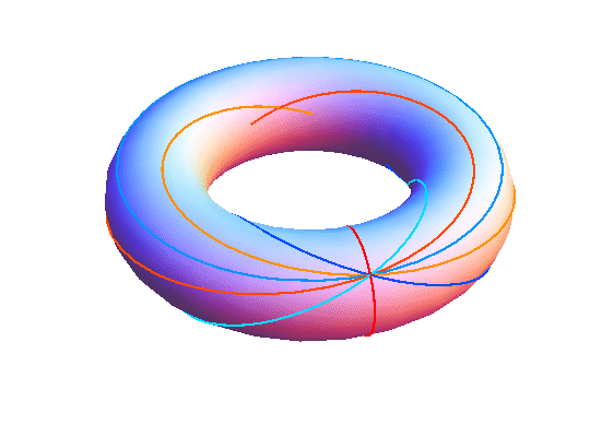
You can draw contour lines of a scalar function on a surface too, optionally with arrows:
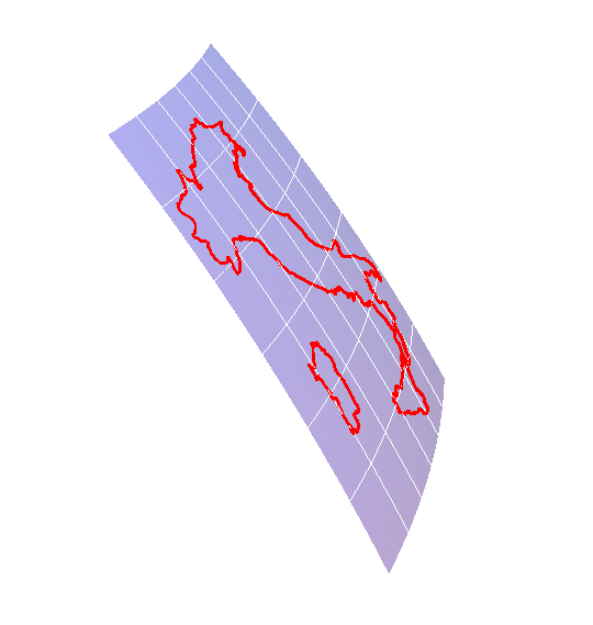
You can draw 3D text on a surface too:


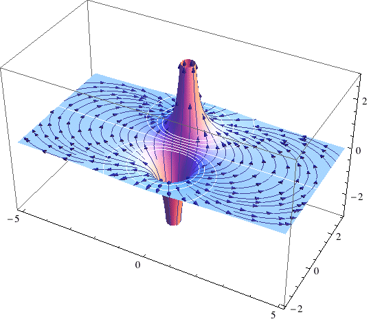
With Mathematica version 7 or later, you can draw stream lines of a vector field onto a surface:
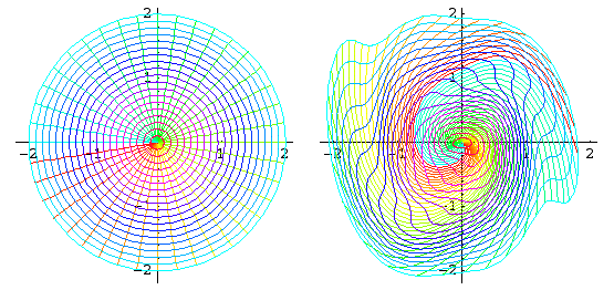
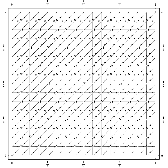
PoincareMaps6 is a package that helps visualize Poincaré map for a plane system of differential equation. The following picture shows on the left a polar grid and on the right the position of the grid after some under the effect of a certain system of the form x'=y, y'=-f(t,x), as computed with the package:
PoincareMaps6 works on Mathematica 6 or later. A version that runs on Mathematica 5.2 or earlier is also available as PoincareMaps.
Latest revision: March 31, 2022.
This Mathematica notebook file defines functions that calculate and plot some notable objects in Real Analysis:
See also the lecture notes (in Italian) on these subjects.
Related MathSource notebooks: The Cantor Set and Mathematica, The Peano Curve, Plotting the Monsters of Real Analysis.
Cantor's set:
Element[1/4, CantorSet]TrueElement[1/2, CantorSet]
FalseCantorSetPlot[{0, 1, 2, 3, 4}]
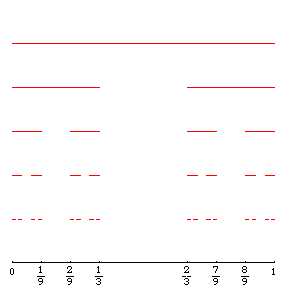
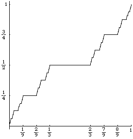
Vitali's function ("Devil's staircase"):
Vitali[1/4]1/3VitaliPlot[0, 1];
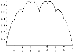
Peano's continuous curve that fills a square (see also this QuickTime movie (700K)):
PeanoCurve[1/5]{1/10, 1/2}PeanoCurvePlot[8];
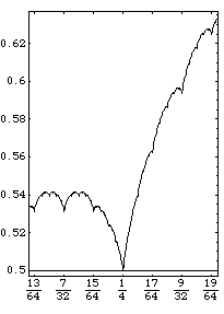
Van der Waerden's continuous, nowhere differentiable function (see the lecture notes):
VanDerWaerden[4/9]40/63VanDerWaerdenPlot[0,1]
VanDerWaerdenPlot[.2,.3]
Latest revision: November 22, 2001.
This Mathematica notebook file defines two routines (PeriodicPlot and PeriodicPlot3D) that help visualizing periodic functions. Tutorial example applications are provided. For example, if you type
PeriodicPlot[Sin[x]+Cos[3x],{x,-2Pi,2Pi}]
you will get the following picture, where a whole period of the graph is automatically highlighted and the tick marks are in multiples of Pi
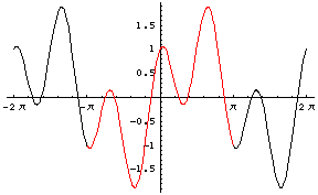
The plot was made with the default settings. You can change the highlighted interval at will. Also, the function need not be periodic: the program automatically takes the values in the highlighted interval and repeats them periodically. For example, to plot a square wave just type PeriodicPlot[Sign[x],{x,-2Pi,2Pi}]
With the following command
PeriodicPlot3D[Re[z^2],z]
you will see a graph of a real-valued function on the unit circle of the complex numbers:
here too the display is customizable with various options.
The Graphic Gallery contains a live rendering and a ray-traced version of similar 3D plots.
Here is a .pdf file (633K) with ready-made pictures made with this package, illustrating Fourier series.
The source code for generating 3D graphs of some functions of 2 variables that are of interest for a beginner in higher calculus. For example the function
has a continuous extension at the origin, and has directional derivatives in all directions, but it is not differentiable. One way to see it is that there are tree directions of maximum slope pointing away from the origin. For differentiable function there is only one (the direction of the gradient).
Chek out this same graph also in its Live3D glory and in its high-definition printable pdf version.